Spectrophotometric Color Calibration
Warning
The calibration of the colors by photometry must imperatively be carried out on a linear image whose histogram was not yet stretched. Otherwise, the photometric measurements will be wrong and the colors obtained without guarantee of being correct.
Spectrophotometric Color Calibration (Ctrl + Shift + C) is the newest method of color calibration available in Siril. This method uses the extensive spectral data available in the Gaia DR3 catalogue [GaiaDR3]. This can be accessed either through direct querying of an online catalogue or by downloading a local extract and querying the local catalogue.
For efficiency and due to the complexity and fragility involved in the original two-step query required to get SPCC data directly from the Gaia Archive, since 1.4.1 the remote catalogue is a hosted copy of the local catalogue. This permits much more efficient querying using HTTP RANGE requests. The master record for the uncompressed catalogue suitable for random access is DOI 10.5281/zenodo.17988558. (Note that since this variant is uncompressed it is not recommended to download entire chunks from this source: for information on installing the local catalogue, see below.)
Warning
Note that if the remote catalogue and all mirrors are offline for maintenance or due to faults, Siril's SPCC functionality will not be available using the remote catalog. Fortunately the primary source (Zenodo) is normally very reliable and the mirror(s) provide backup, however a status indicator is built into the SPCC dialog. The remote catalogue status is checked when the dialog starts up and can be re-checked by clicking the status button.
The offline Gaia SPCC extract will still work fine if the remote catalogue is unavailable.
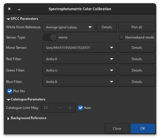
SpectroPhotometric Color Calibration dialog window.
Tip
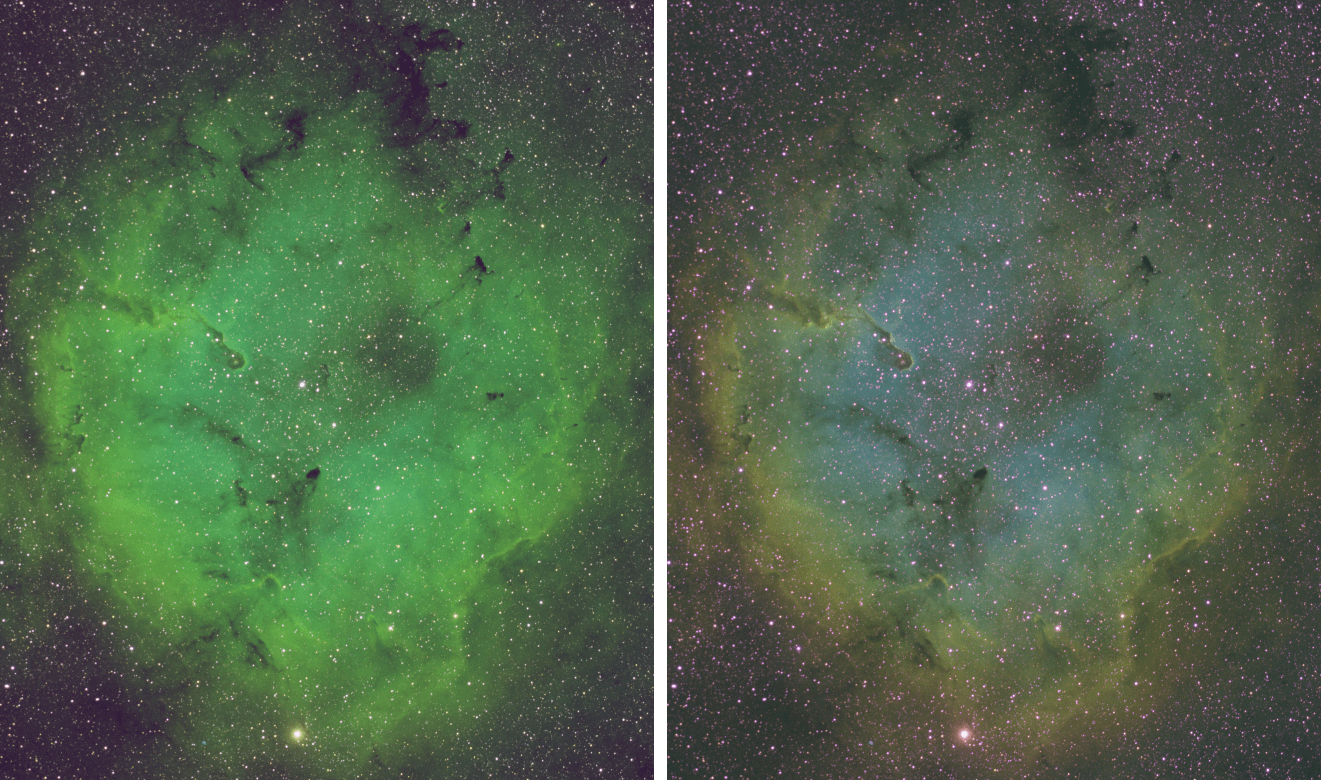
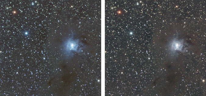
What's the difference between SPCC and PCC? When should I use one rather than the other? SPCC is a more accurate version of PCC and renders the latter obsolete. SPCC takes your setups sensor and filters into account. As a result, the color produced is closer to "reality". The example in the picture below illustrates the difference in results.

Comparison between PCC (left) and SPCC (right): click to enlarge. (Courtesy of Ian Cass)
Local SPCC Catalog
From 1.4.0 an offline SPCC catalog is available using Gaia DR3 data. Note that the catalog is chunked into 48 files covering each level 1 HEALpixel.
Theory
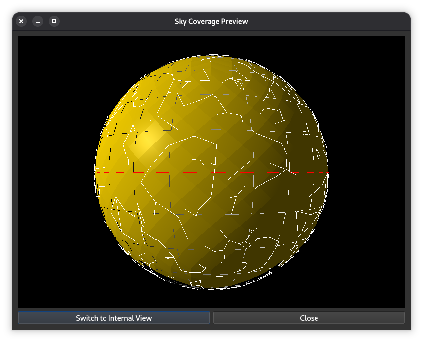
HEALpix (Hierarchical Equal Area isoLatitude Pixelisation) is an algorithm for pixelising a sphere based on subdivision of a distorted rhombic dodecahedron. Mathematical details can be found on Wikipedia [Wiki_HEALPIX]. Gaia sources use a Level 12 NESTED HEALpix scheme and the HEALpixel number is encoded into the source_id. The specification of the Gaia DR3 catalogue extracts and their file format is documented here (PDF).
The nested nature of the scheme means that HEALpixels that are close together in the sky have numbers that are close together. The hierarchical property also means that it is possible to index sources in HEALpixels at a deep HEALpixel level and divide the catalog into chunks at a shallower level while still supporting a highly efficient catalog search algorithm.
It is possible to download the entire catalog or only the chunks you need. The folder location to store the catalog files is set in .
Sirilpy script
The easiest way to install the catalog is to use the built-in Python script
Siril_Catalog_Installer.py in the menu.
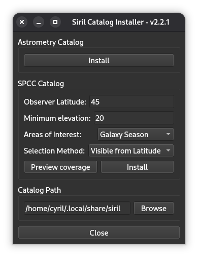
This provides an interface that allows you to install either the whole catalog, or only the chunks that are visible from your observing latitude above a certain elevation, or only sets of chunks corresponding to certain themes (Milky Way, Summer Triangle, Galaxy Season etc.) Select the latitude / elevation or area of interest if desired, and then select the selection method (All, Visible from Latitude or Area of Interest).
You can preview the coverage using the Preview coverage button.
Finally, clicking Install will download, verify, uncompress and install the selected chunks and also set the catalog path in Siril's preferences. A default catalog path is suggested in the text entry widget, but can be changed to a different location if you prefer.
If you wish to install the offline SPCC catalog files manually, they can be downloaded from DOI 10.5281/zenodo.14697692. Either individual level 1 HEALpixels can be downloaded or the entire catalog can be downloaded as an archive.
Tip
When you download "All Files" from the Zenodo record, the download is a zip archive that you will need to extract, however the zip archive is just a convenient way of bundling all of the individual files; the data files inside the zip archive are themselves compressed with bzip2 compression, and you will need to decompress the individual .bz2 files before Siril can use them. Support for this compression format is available by default in Linux and MacOS, and is provided in Windows by various archive programs including 7-Zip and Pea-Zip, which are both Free and Open Source software.
All compressed files have accompanying sha256sums and there is a file containing all the sha256sums of the uncompressed files as well, for additional validation. The Zenodo record also provides a DOI reference that can be used to cite the dataset if you use it in academic work.
Siril uses an optimized extract of the Gaia DR3 xp_sampled datalink product. As with the astrometric extract, the offline catalogue is capped at the 127 brightest sources per level 8 HEALpixel. The catalogue contains fewer sources than the astrometric extract as xp_sampled spectra are typically only provided for sources brighter than magnitude 17.6 and therefore more HEALpixels in emptier parts of the sky have fewer than 127 sources compared with the astrometric extract (i.e. these HEALpixels contain all the available Gaia DR3 sources with xp_sampled data), but this approach still avoids overpopulation of the catalogue in extremely crowded parts of the sky while providing the best SNR. In those HEALpixels with fewer than 127 xp_sampled sources, the local catalog is as comprehensive as using the online Gaia archive directly.
The xp_sampled is converted from float32 to float16 data with an additional byte setting the exponent to be applied to the xp_sampled data for the source to overcome limitations on exponents expressible with float16. This is entirely justifiable given the error bars on the xp_sampled data and makes no practical difference to the accuracy of the results. It means that we can provide a highly effective, purpose-optimized local SPCC catalogue in under 21GB of data.
How it Works
SPCC requires knowledge of your sensor and the RGB filters you use. These are provided through an online repository which Siril will sync, either automatically at startup or manually when required. Sensor and filter information is updated via the same synchronization method as used for the online scripts repository. (This means that as data on new filters or sensors becomes available it can be added to the repository without requiring an update to the application.)
In the GUI you select your sensors and filters from the widgets in the SPCC dialog. Don't worry if there isn't an exact match for your equipment, just pick the closest option, or the appropriate default option. You also need to select a white reference. The default reference is the Average Spiral Galaxy reference which is suitable for a wide range of astrophotographic scenes, however there is an extensive range of galaxy and star types to choose from. The Sun's spectral type is G2(v) so if you want to balance your image using sunlight as a white reference, you would pick Star, type G2(v) from the list.
SPCC then uses the stellar spectra in Gaia DR3 and knowledge of your imaging sensor and filters to compute for each star in the catalogue that matches a star detected in the image by Siril the expected flux in each color channel. It then compares this with the actual flux measured in each channel using Siril's photometric capabilities.
Given the sensor and filter knowledge, SPCC computes the expected flux in each channel for the specified white reference. A robust linear fit is obtained to give the best fit of catalogue to image R/G and B/G flux ratios for each star and for the white reference. This fit is used to derive correction coefficients which are applied multiplicatively to each channel, resulting in spectrophotometrically accurate color channels.
Your image must be plate solved for SPCC to work: if it is not already, this should be done with the dedicated tool. It is important to make sure that the plate solving information is correct, as some software is known to add inaccurate WCS data to images.
Graphical Interface
Selection of Sensor In order to select your sensor, ensure that the mono / OSC toggle button is set correctly. You will then see the appropriate dropdown to choose from the available sensors.
Selection of Filters SPCC can operate in two modes.
The default mode is broadband operation. In this mode, the Narrowband mode check box should be unchecked. You can choose either red, green and blue filters (for composited images made with a mono sensor) or OSC filters, for example light pollution filters, for images made with an OSC sensor.
Warning
If you select a DSLR OSC sensor (e.g. a Canon EOS 600D) an additional widget will become visible to select a DSLR Low Pass Filter. This allows you to tailor whether your camera has been astro-modded or not. You must select an option here or the process will complain that you haven't set all the necessary filters!
Options exist for Canon and Nikon OEM low-pass filters as well as the popular Baader BCF astro-mod filter that lets Ha and Sii through but still blocks longer IR wavelengths and "Full spectrum" which is modelled as a perfect clear filter.
If you have an unmodified camera of a different model or brand, select any of the Canon or Nikon low-pass filters: the effect is very minor as these wavelengths are right at the edge of human visual perception anyway.
By checking the Narrowband mode check box, you enable narrowband mode. This is intended either for images composited from narrowband filters used with a mono sensor or for images made using an OSC sensor with a dual, tri-band or quad band narrowband filter. In this mode the available controls change, and for each color channel you enter the nominal wavelength and bandwidth of the filter passband. For ultra-narrowband mono filters the passband may be as little as 3nm; for a quadband OSC filter like the Altair QuadBand V2 the passbands may be as much as 35nm. Note that for a HOO composition where two channels are set to the same data, the nominal wavelength and bandwidth should be set equal in the SPCC interface too.
Calibrated HOO image. Image by Cyril Richard.
Tip
Some manufacturers specify a center wavelength and FWHM. It is fine to use the FWHM as the bandwidth: these filters have very sharp cutoffs.
Warning
Don't expect to retrieve the Hubble palette for SHO imaging using the wavelengths of the SII, \(\mathrm{H}\alpha\) and OIII filters respectively. The result will be an image with a huge green cast. This is easily explained by the fact that the SII emission line is much fainter than that of hydrogen, and the SPCC gives a representation of real intensities. But this is not the case in the Hubble palette. In fact, manual color calibration will give better results.
SHO image calibrated by SPCC compared to the same, manually calibrated one. The entire nebula was taken as a white reference during manual calibration. Image by Cyril Richard.
Selection of DSLR Low Pass Filter (LPF) DSLRs contain a low-pass filter (sometimes also called a 'hot mirror'. These reduce transmittance at wavelengths of interest to astronomers (Ha at 656nm and S-II at 674nm). If the selected OSC is a DSLR, a dropdown will be provided from which you can the appropriate LPF profile. Options exist for stock LPFs as well as astro-modified LPFs and an ideal Full spectrum filter model for if the LPF has been removed altogether.
Selection of White Reference SPCC requires an absolute white reference spectrum. The default is Average Spiral Galaxy and the source spectra used to create this white reference are taken from the SWIRE templates [SWIRE] in a manner consistent with other astrophotography software providing the same white reference. A wide range of other white references is available, covering the full range of galaxy and star classifications [Stellar]. If you wish to use sunlight as your white reference, you would choose the white reference Star, type G2(v) as the Sun is a type G2(v) star.
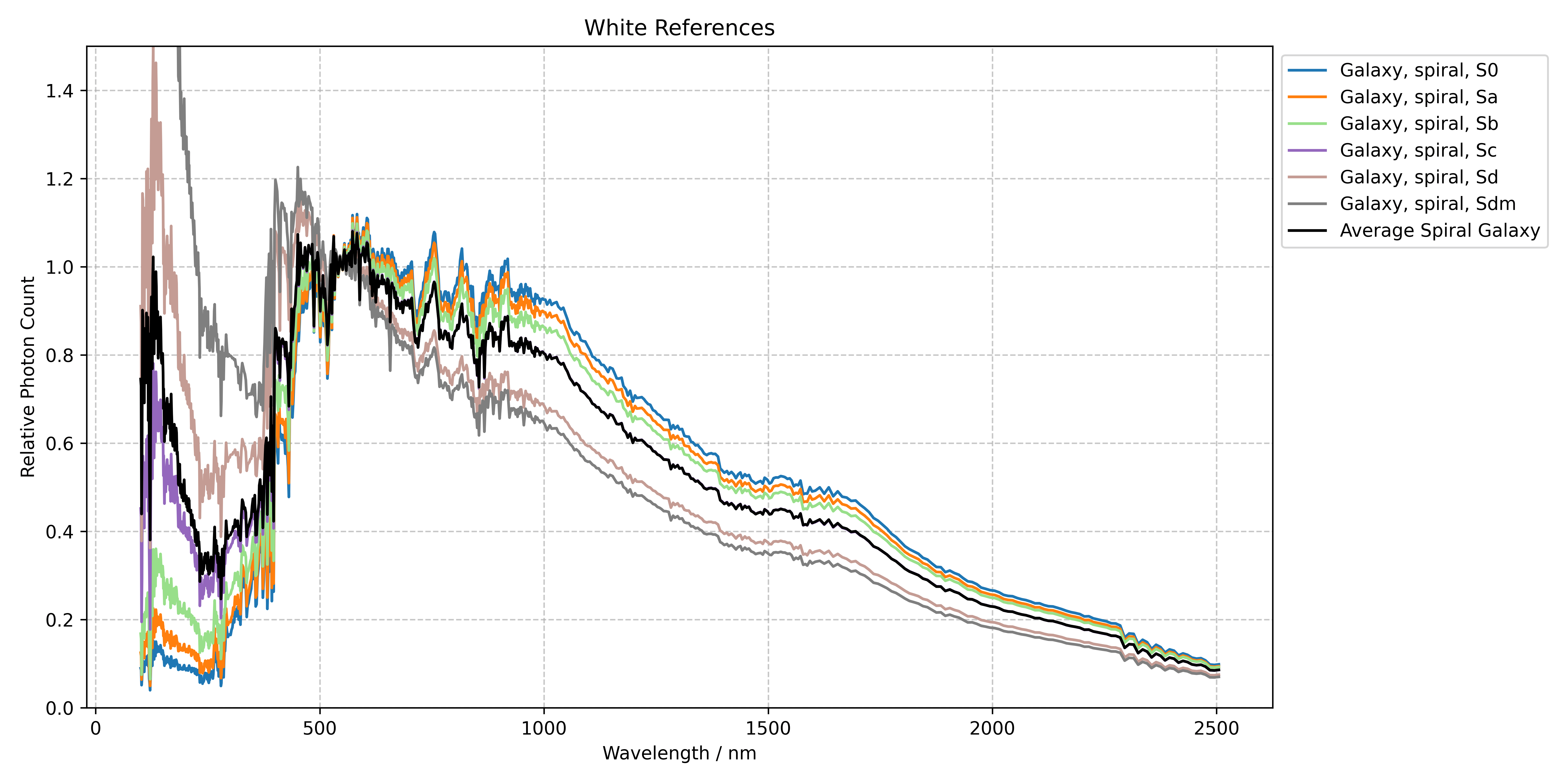
Graphs showing white reference data from spiral galaxies. At around 350 nm, the Average Spiral Galaxy data become identical to the Sc galaxies, which are also a good representation of the white reference.
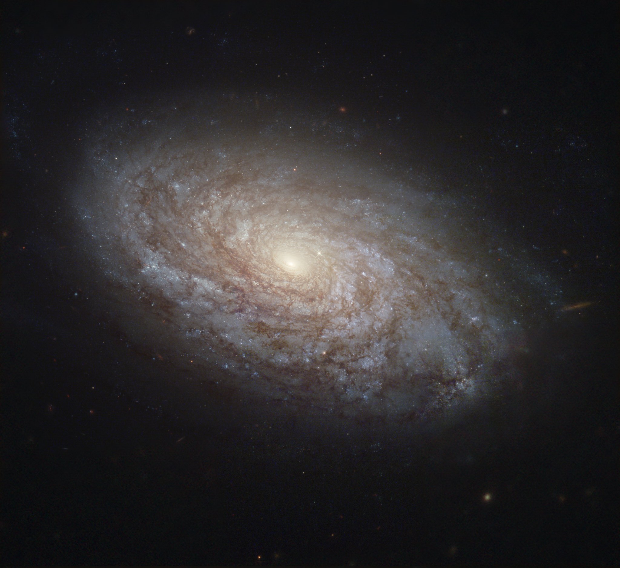
NGC 4414 is a great example of a Sc-type galaxy, the type closest of the average spiral galaxy used as white reference by default. Image Credit: NASA, ESA, W. Freedman (U. Chicago) et al, & the Hubble Heritage Team (AURA/STScI), SDSS; Processing: Judy Schmidt.
Tip
Summary of Stellar Spectral Classifications Stellar classifications have two parts, a Morgan-Keenan type and a Luminosity index.
The first part of the spectral classification (G2 in the case of the Sun) takes one of the following letters: O, B, A, F, G, K, M. O represents extremely hot blue stars, while M represents cool red stars. The sun is roughly in the middle of the spectrum. The number represents intermediate cases, for example a B5 star is halfway between type B and type A.
The second part of the spectral classification is the luminosity index ranging from i to v. Stars with luminosity index i are supergiants, whereas stars with luminosity index v are dwarfs. Main sequence stars such as the sun have a luminosity index of iv.
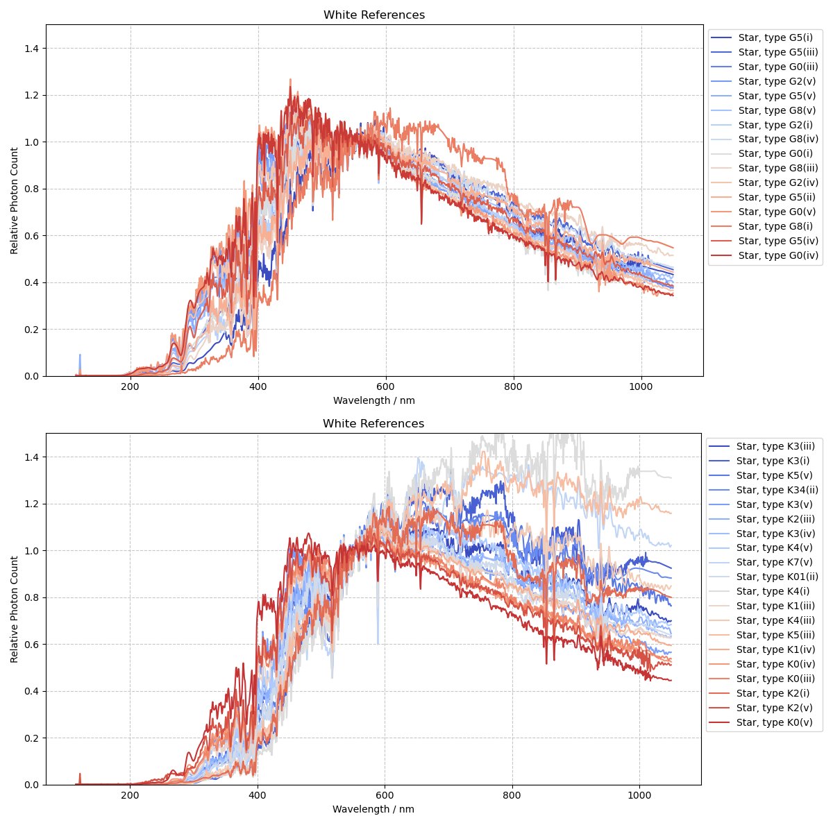
Graphs showing white reference data for a set of two different star classes, G and K.
Difference in color calibration depending on the choice of white reference. On the left, an M-type star, on the right the average spiral galaxy. Please note that the data are linear, and only an autostretch has been applied to the visualization.
Atmospheric Correction Siril's SPCC supports atmospheric correction. When imaging from Earth we image through the atmosphere. This does not have perfect transmittance and therefore acts as another, non-optional, filter in the imaging chain between the sensor and the astronomical object. Whether or not to correct for this is an artistic choice each astrophotographer must make, but the option is provided.
Theory
Atmospheric extinction arises from several sources. The most important are:
Rayleigh scattering. This is the elastic scattering of light by particles that are small compared with the wavelength of light. The strong wavelength dependence of the Rayleigh scattering (\(\approx λ^{−4}\)) means that shorter (blue) wavelengths are scattered more strongly than longer (red) wavelengths.
Aerosol scattering. This is scattering of light by particles that are larger than the wavelength of light. This is quite variable but (in the absence of significant short term dust or smoke effects) relatively spectrally flat and less significant than Rayleigh scattering.
Molecular absorption lines.
Siril models only Rayleigh scattering. This is the most important contribution in most atmospheric conditions, and is highly predictable making it easy to model without requiring the user to provide complex data.
The formula for the Rayleigh transmittance of the atmosphere as a function of wavelength \(\lambda\) nm, observer height \(H\) m and pressure \(p\) hPa is:
\(\tau_R(\lambda, H, p) = \left( \frac{p}{1013.25} \right) \left( 0.00864 + 6.5 \times 10^{-6} \cdot H \right) \lambda^{-(3.916 + 0.074 \lambda + \frac{0.050}{\lambda})}\).
Under normal circumstances aerosol scattering has a roughly flat response in the visible region. This changes in specific conditions, for example when there is high atmospheric smoke particle concentration after wildfires or, in parts of Europe, when Saharan dust is carried into the atmosphere. However these effects are very difficult to model accurately as they depend on the concentration of sand or smoke particles in the atmosphere at the time. Siril therefore does not model this effect.
The main molecular absorption lines in the visible spectrum are the Chappuis stratospheric ozone bands and the Fraunhofer B molecular oxygen absorption line. However the Fraunhofer B line is very narrow and does not have a significant effect on overall calibration. The Chappuis bands are broad but with a low peak absorption, with a much smaller overall impact than Rayleigh scattering. Molecular absorption bands are not currently modelled in Siril.
When selecting the Atmospheric correction check box, the following options become available:
Observer Height. This allows setting of the observer height, which is used in the Rayleigh extinction calculation. Set this to the altitude of your observatory above sea level. Some capture software sets the FITS header
SITEELEVcard: if this is present, the height from this card will be used, otherwise the value is editable and defaults to 10 m.Atmospheric pressure. This allows setting atmospheric pressure at the time of observation. For convenience it can be specified as sea level pressure (as provided by weather forecasts) or as local pressure (as measured by a barometer at the observatory). In case you are unsure, the default is standard atmospheric pressure at sea level (1013.25 hPa).
Theory
If the pressure is provided as a sea-level pressure measurement, the local pressure at the observer's height is calculated according to the barometric formula:
\(P(h) = P_0 \left( 1 - \frac{L h}{T_0} \right)^{\frac{g M}{R L}}\),
where:
\(L = 0.0065~\text{K}/\text{m}\) (Temperature lapse rate),
\(T_0 = 288.15~\text{K}\) (Sea level standard temperature),
\(g = 9.80665~\text{m}/\text{s²}\) (Acceleration due to gravity),
\(M = 0.0289644~\text{kg}/\text{mol}\) (Molar mass of Earth's air),
\(R = 8.3144598~\text{J}/(\text{mol}·\text{K})\) (Universal gas constant).
Airmass. This is not an editable parameter but shows the airmass that will be used in the calculations. It is obtained, in order of preference, from the
AIRMASSFITS header card; by calculation using theCENTALTFITS header card; or as a last resort by using the average zenith angle of all parts of the more than 30° above the horizon. The tooltip shows which source the used figure is based on.Theory
If the
AIRMASSheader is unavailable the calculation used to derive airmass from zenith angle is calculated in accordance with [Young1994]:\(X(z) = \frac{1.002432 \cos^2 z + 0.148386 \cos z + 0.0096467}{\cos^3 z + 0.149864 \cos^2 z + 0.0102963 \cos z + 0.000303978}\).
The interface allows you to view details of the selected sensor, filter and white reference using the Details button next to each combo box. From the details information box that this brings up you also have the option to plot the Quantum Efficiency (for sensors) or transmittance (for filters) or relative photon count (for white references) against wavelength. A Plot All button is also available in the main SPCC dialog which allows you to see the responses of all your filters and your sensor and the white reference spectrum all plotted together.

Plotting all the responses of all your filters and your sensor and the white reference spectrum all plotted together
When you are happy, click Apply and SPCC will run. It will cache catalogue data but the first time you apply it to an image it will take a few seconds to perform the online catalogue searches and retrieve the source and spectral data. SPCC will then be applied to the image. Additional plots showing the linear fit of the catalogue Red / Green and Blue / Green to image Red / Green and Blue / Green ratios.
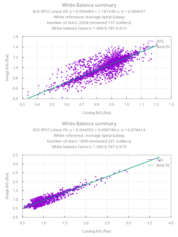
By default, Siril outputs graphs showing the fits used in the process. In this example the magnitude was limited to 17.
Tip
How do I process L-RGB images? We recommend processing only RGB with SPCC. The L layer must be added at a later stage, when the histograms have been stretched.
Tip
For images taken with an OSC sensor, we recommend using Bayer Drizzle to recover image colors. This ensures more accurate colors as shown in the following image.

SPCC applied identically to the same image. On the left, conventional demosaicing using the VNG algorithm; on the right, the Bayer Drizzle technique. A dominant green hue is clearly visible on the conventionally demosaiced image. Note that the VNG algorithm was chosen for this example because the effects explained here are more pronounced. However, in Siril, the default demosaicing algorithm is RCD. Click to enlarge image.
SPCC filter and sensor database
Converting the Data
The format used for the database is JSON (a lightweight data-interchange format derived from JavaScript object notation). We recommend starting with an existing file from the database that suits your needs and saving it under the name of your sensor or filter. You can then simply replace the values in the file with the data you have obtained.
In the
wavelengtharray, enter your wavelength measurements. Make sure to properly set theunitsfield to one of the following values:angstroms,nm,micrometres, orm.In the
valuesarray, enter either:Transmittance values for filters
Quantum efficiency values for sensors
Set the
rangefield according to your data scale (e.g.,"range": 100if your values are percentages,"range": 1if they are normalized to 1).
How to Contribute
The SPCC database is designed to store JSON files of OSC/monochrome sensors and filters available in the market. Its primary objective is to gather extensive data, fostering collaboration within the community.
We greatly value community contributions and encourage active participation. We are in need of data spanning ideally from 300nm to 1100nm. Software tools can be employed to extract curves/charts found online, and contacting manufacturers directly for data is also an option.
Read this page and help us by contributing.
Important
We do not include narrowband filters. These highly specific filters are synthesized in Siril, ensuring precision. This also applies to duonarrowband filters.
JSON File Format Reference
Here is the template for the JSON files used in the SPCC database:
[
  {
    "model": "sensor model / filter set",
    "name": "sensor / filter name",
    "type": "MONO_SENSOR | OSC_SENSOR | MONO_FILTER | OSC_FILTER | OSC_LPF | WB_REF",
    "dataQualityMarker": 1 - 5,
    "dataSource": "Describe where the data came from",
    "manufacturer": "Manufacturer name",
    "version": 1,
    "channel": "RED | GREEN | BLUE | LUM",
    "wavelength": [Comma separated array of wavelengths],
    "values": [Comma separated array of values]
  }
]
Important Notes
Definition of the
dataQualityMarkerfield:Data of unknown provenance. Not accepted for the siril-spcc-database repository.
Data scanned from OEM or other reputable plots in image format.
Lower resolution tabulated data provided by the OEM, or academic data relating to ideal standard filter transmittance (e.g. generic standard photometric filters).
High resolution (no more than 2nm spacing) tabulated data provided by the OEM.
Data specific to your own filter which you have personally calibrated using appropriate equipment. This is the highest possible quality marker and will never be given to .json files in the repository which can only ever be generic to an equipment model, not specific to your individual equipment item. Note that the actual quality of this data is entirely dependent on the quality of your calibration equipment - the old adage "garbage in, garbage out" applies.
The
modelname requirements:Must be identical for all related JSON objects in a set
Examples:
RGB filter set:
"model": "Chroma RGB"OSC sensor:
"model": "ZWO ASI2600MM"
The
channelfield:Required only for
"type": "OSC_SENSOR"or"type": "MONO_FILTER"For OSC sensors, include one JSON object per channel (
RED,GREEN,BLUE)Preferred channel order:
RED,GREEN,BLUE
The
wavelengtharray requirements:Minimum coverage: 380nm to 700nm
Maximum useful range: 336nm to 1020nm (Gaia DR3 spectra limits)
Values must be monotonically increasing
No duplicate values allowed
Must use specified units (
angstroms,nm,micrometres,m)
Note
If your sensor data only extends down to 400nm (which is common with some manufacturers), it is acceptable to extrapolate a single point at 380nm. The sensor response below 400nm typically follows a predictable pattern across different sensors. Adding this extrapolated point at 380nm is preferable to letting the curve end at 400nm, which would effectively treat all response below 400nm as zero. The impact of this extrapolation is minimal since the CIE 1931 response is very low in this wavelength range.
The
valuesarray requirements:For filters: contains transmittance values
For sensors: contains quantum efficiency values
Set appropriate
rangevalue (e.g., 100 for percentages)Siril scales all values to 0.0-1.0 range internally
Saved Preferences
As most users are likely to do most of their imaging with one setup, or maybe two, it would be tedious to reselect the sensor and filters each time. The user choices are therefore automatically remembered when set and restored next time the tool is used, even if Siril is closed and restarted in between. This works using the preferences system but there is no need to use the preferences dialog to remember the set sensor and filters, it is done automatically.
The chosen white reference is not remembered: the default Average Spiral Galaxy is a suitable choice for most astronomical scenes, and alternative white references would normally be set for a specific image to draw out a particular aspect of the color.
Siril command line
spcc [-limitmag=[+-]] [ { -monosensor= [ -rfilter= ] [-gfilter=] [-bfilter=] | -oscsensor= [-oscfilter=] [-osclpf=] } ] [-whiteref=] [ -narrowband [-rwl=] [-gwl=] [-bwl=] [-rbw=] [-gbw=] [-bbw=] ] [-bgtol=lower,upper] [ -atmos [-obsheight=] { [-pressure=] | [-slp=] } ]
spcc_list { oscsensor | monosensor | redfilter | greenfilter | bluefilter | oscfilter | osclpf | whiteref }
References
Vallenari, A., et al. "Gaia Data Release 3-Summary of the content and survey properties." Astronomy & Astrophysics 674 (2023): A1. 99(613), 191.