Image are stored as pixel values that come from the camera following a
quasi-linear law, meaning that for areas of the sky that show no visible
feature, the pixel value will be close to zero, but for bright objects like
stars it will be close to a maximum value depending on exposure and gain. In
between, if a nebula has a surface magnitude half of a star, it will have pixel
values half of those of the star and so on. This is what we call the linear
pixel mode.
The human eye doesn't quite see photons like that. It amplifies dark areas,
so that an object maybe a tenth as bright as another would look half as bright.
For astronomy images, we usually display images with a similar pixel value
scaling (see display modes from the GUI).
But it is only a display trick, using a screen transfer function, to render
the pixel values of the untouched image to better looking images.
Image stretching is about doing something similar but by modifying the pixel
values of images instead of just altering their rendering. Siril has three main
tools to achieve this.
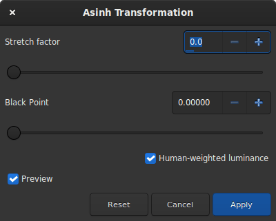
The asinh, or inverse hyperbolic sine, transformation will modify image pixel
values in a way similar to what can be seen with the asinh display pixel
scaling function, which is parametrized by the low and high values cut-off
cursors. Here the parameters are the stretch factor and the black point value.
where rgb_original is computed using the pixel values of the three channels.
A clipping mode can also be set.
Theory
As rgb_original is an average of the 3 channels, one or two channel values
will be greater than rgb_original and can therefore clip. This can cause color
artefacts when bright, strongly-colored regions are stretched. In order to
avoid this problem the RGB blend clipping algorithm was developed by the
authors of the original GHSastro tool: the same algorithms are available in
the Siril implementation and this is the default clipping mode for stretches
that require handling of clipping. The \((r, g, b)\) values are stretched first
based on the luminance value rgb_original to give \((r', g', b')\). Then
the original \((r, g, b)\) values are independently stretched to give
\((r'', g'', b'')\). Finally the largest value of \(k\) is identified
such that
\(k \times r' + ( 1 - k ) \times r'' ≤ 1\);
\(k \times g' + ( 1 - k ) \times g'' ≤ 1\);
and
\(k \times b' + ( 1 - k ) \times b'' ≤ 1\)
Then the transformed values are calculated as
\(( k \times r' + ( 1 - k ) \times r'', k \times g' + ( 1 - k ) \times g'', k \times b' + ( 1 - k ) \times b'')\)
This RGB blend clipping algorithm is also available for the Generalised Hyperbolic
Stretch transforms described below.
Other choices of clipping algorithm are available:
Clip - this clipping mode just allows any colour components that clip to
clip, but restricts them to values in the range 0.0 to 1.0. This may suffer
from coloured artefacts such as fringes around nearly-saturated stars, but
it is extremely quick to calculate.
Rescale - this clipping mode checks the R, G and B components of each
pixel and if any are > 1.0 it rescales the pixel so that no components are
clipped. This method is prone to artefacts and is mainly included for feature
equivalence with the GHSastro plugin. It is quick to compute.
Global Rescale - this clipping mode behaves similarly to Rescale except
that the scaling is computed globally instead of per-pixel. This avoids
the kind of artefacts that Rescale can produce, but has a bigger impact on
overall image brightness. This is faster than RGB blending to compute
but slower than Clip or Rescale.
When the Use Human-weighted Luminance option is not ticked, rgb_original is the
mean of the three pixel values; when it is set, weighting changes to 0.2126
for the red value, 0.7152 for the green value and 0.0722 for the blue value,
which gets results closer to human perceptual color balance.
Stretches the image to show faint objects using an hyperbolic arcsin transformation. The mandatory argument stretch, typically between 1 and 1000, will give the strength of the stretch. The black point can be offset by providing an optional offset argument in the normalized pixel value of [0, 1]. Finally the option -human enables using human eye luminous efficiency weights to compute the luminance used to compute the stretch value for each pixel, instead of the simple mean of the channels pixel values. This stretch method preserves lightness from the L*a*b* color space. The clip mode can be set using the argument -clipmode=: values clip, rescale, rgbblend or globalrescale are accepted and the default is rgbblend. This command is mask-aware and will obey the mask if and only if the -mask flag is provided
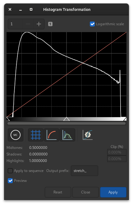
The tool is presented in the form of a histogram with 3 sliders (in the form
of a triangle placed underneath) that we must move to transform the image.
The triangle on the left represents the shadow signal, the one on the right
the highlights and finally, the one in the middle the midtone balance
parameter. The values of these sliders are displayed below the histogram, on
the left, and can be changed directly by hand. Opposite is the percentage of
pixels that are clipped by the transformation: it is important not to clip too
many pixels. If only the midtones parameter is changed, then no pixel can be
clipped.
Theory
The new pixel values are then computed with this function:
It is generally not recommended to change the value of the highlights,
otherwise they will become saturated and information will be lost.
The toolbar contains many buttons that affect the visualization of the
histogram. You can choose to display the input histogram, the output
histogram, the transfer curve and the grid. The button
allows you to apply the same transformation as the autostretch algorithm. It
is rarely advisable to use this button as is. Adjustments are usually
necessary to avoid losing information.
Tip
When the button is pressed, the sliders and
lo, mid and hi entries will become temporarily inactive. You have to apply
the autostretch with the Apply button and the controls will
reactivate. You can then apply adjustments as a second follow-up stretch.
This behaviour avoids problems where the monitor ICC profile is different
to the image ICC profile.
At the top of the histogram it is also
possible to choose to display the histogram in logarithmic view, as in the
illustration. This behavior can be made default as explained
here. Finally a zoom in X
is available. This is very useful when all the signal is concentrated on
the left of the histogram.
Tip
If a ROI is set, the MTF histogram preview will not update to show the impact
of the stretch on the ROI. This is because that behaviour could be misleading:
if the ROI is not typical of the image overall, adjusting the ROI histogram
to a suitable level would result in a badly adjusted histogram for the
overall image and potentially a burned-out or excessively dark look to the
result. When in ROI mode the stretch parameters should be adjusted by eye.
If it is desired to check the histogram for the stretch as applied to the
image as a whole, the ROI should be cleared.
Siril command line
mtf low mid high [channels] [-mask]
Applies midtones transfer function to the current loaded image.
Three parameters are needed, low, midtones and high where midtones balance parameter defines a nonlinear histogram stretch in the [0,1] range. For an automatic determination of the parameters, see AUTOSTRETCH.
Optionally the parameter [channels] may be used to specify the channels to apply the stretch to: this may be R, G, B, RG, RB or GB. The default is all channels. This command is mask-aware and will obey the mask if and only if the -mask flag is provided
Auto-stretches the currently loaded image, with different parameters for each channel (unlinked) unless -linked is passed. Arguments are optional, shadowclip is the shadows clipping point, measured in sigma units from the main histogram peak (default is -2.8), targetbg is the target background value, giving a final brightness to the image, range [0, 1], default is 0.25. The default values are those used in the Auto-stretch rendering from the GUI.
Do not use the unlinked version after color calibration, it will alter the white balance. This command is mask-aware and will obey the mask if and only if the -mask flag is provided
Applying transformation to the sequence
This transformation can easily be applied to a sequence. You just have to
define the transformation on the loaded image (with a sequence already loaded),
then check the Apply to sequence button and define the output prefix of
the new sequence (stretch_ by default), or use the following command:
Siril command line
seqmtf sequencename low mid high [channels] [-prefix=]
Same command as MTF but for the sequence sequencename.
The output sequence name starts with the prefix "mtf_" unless otherwise specified with -prefix= option
This is the most capable and modern tool of Siril, also the most complex to
learn. A very detailed tutorial for this tool in Siril was written by the
authors of this algorithm: https://siril.org/tutorials/ghs. Here, we
will just summarize here the basic operation of this tool.
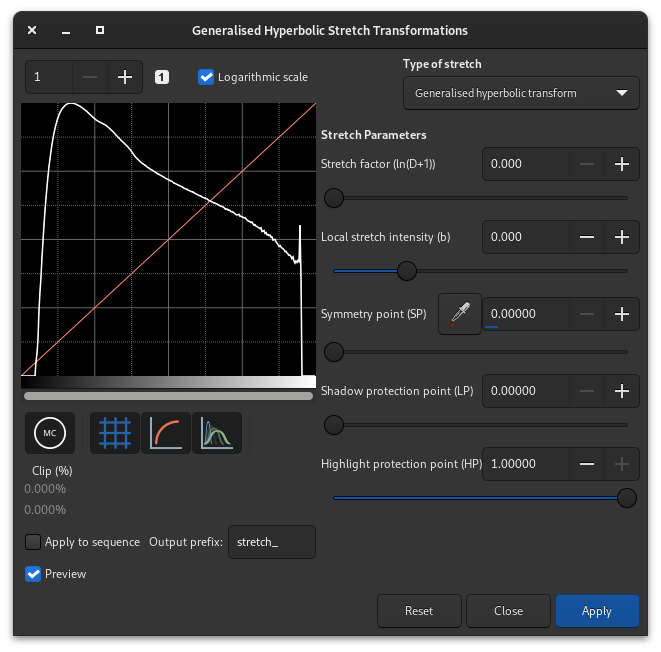
Simply put, the GHS is able to improve the contrast of a range of brightness
levels in an image. For example, if one wanted to better view the details in
the medium to high brightness part of a nebula (which is in general very faint
in an astronomy image), it would be possible to only select this range for
stretching. It is very good at improving the contrast of main objects without
making stars too big. The tool is very much based on iterative use, so
stretching all the different ranges of brightnesses in the image one after the
other, by small touches.
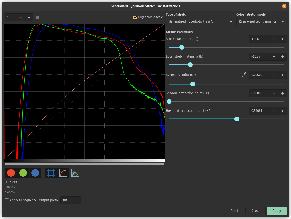
To achieve this, the tool relies heavily on histogram display and interaction,
for each color channel. The transformation function, shaped like a hyperbole or
an 'S', can be altered by moving its center (the SP - symmetry point
parameter), by flattening either of its ends (with shadow and highlight
protections), and of course its twist (stretch D and local stretch b
factors). Manipulating these parameters on a small (for speed) image with an
SP value of 0.5 will help you understanding their effect.
There are two main operations to do on each iteration: selecting the range of
lights to modify, and actually modifying it. Selecting the range is quite easy,
it's a matter of finding a representative value (SP) and defining the width of
the range (b). Setting SP can be done in three ways:
selecting an area of similar brightness in the image and clicking on the
picker button
clicking on the histogram itself with a single leftclick (it is possible to
zoom in the histogram using the + button at the top left)
using the cursor or its associated plus and minus buttons or direct value.
The width of the range depends on the local stretch. A high value of b will
make a small range, and increase contrast over a small range of brightnesses in
the image.
Modifying the histogram once the location of the change has been set is a more
complex operation. One goal given by the algorithm's authors is to make the
logarithmic view of the histogram (enabled by checking the box) as close as
possible to a decreasing line. To do this, bumps need to be carved out and
valleys to be filled. Here is a quick guide of values to use depending on what
needs to be achieved:
initial stretch from linear: set SP slightly to the left of the main
peak, moderate b value from 6 and up, increase D slightly only to
start to see the main object. Do not stretch too much at this point like an
autostretch would do, otherwise the stars would grow too big (main tutorial
section for this).
improving contrast of a range, or filling a valley: set SP to the
centre of the valley in the histogram, set b as high as how narrow the
range or valley is, decrease HP to preserve stars, increase D slowly
until the improvement appears.
decreasing contrast of a range, or flattening a peak: decreasing a peak
is not easy to do but will happen as a side effect of valleys being filled.
For example, creating a peak, or filling a valley, will decrease what is on
the left of SP. Another possibility is to use the inverse transformation,
from the Type of stretch combo box, and a high LP value, and HP at
1.
move curve to the left, making the image darker: often if we stretched
the entire histogram, the peak will move to the right, making the background
too bright. There is a simple way to just move everything to the left, select
in the Type of stretch combo box the last entry, Linear stretch (BP
shift). There's only one cursor to move now, controlling how much it will
shift.
Tip
If a ROI is set, the GHT histogram preview will not update to show the impact
of the stretch on the ROI. This is because that behaviour could be misleading:
if the ROI is not typical of the image overall, adjusting the ROI histogram
to a suitable level would result in a badly adjusted histogram for the
overall image and potentially a burned-out or excessively dark look to the
result. When in ROI mode the stretch parameters should be adjusted by eye.
If it is desired to check the histogram for the stretch as applied to the
image as a whole, the ROI should be cleared.
Some operations are also common for color images, where we often want to
have a similar shape of curve for the three channels, working on each channel
independently by unselecting them with the three colored circles below the
histogram view:
The Generalized Hyperbolic Stretch with a color image
moving the peak to the right: a simple stretch with a SP value left of
the peak will do that in general, so this should be done as part of a
stretch.
spreading a peak: to stretch a channel a bit more and it give it more
importance in the final result, without changing the location of the peak too
much, set SP near the peak or slightly to its right, set b depending
on how the contribution is expected throughout the channel, between a
negative value if the impact shall be felt up to the stars levels (to change
their color) and a high value if this is only for a nebula, increase D to
obtain the target width of the peak, and
then offset the peak to the left by decreasing HP.
moving all channels together: an alternative luminance mapping stretch
exists, see the Color stretch model combo box at the top right of the GHS
window, using either luminance stretch values will stretch the luminance and
reapply colors on it instead of stretching directly the three channels. The
luminance modes can be better at preserving colours in the image. These modes
use the same RGB blend clipping mode described above to prevent color channel
clipping artefacts.
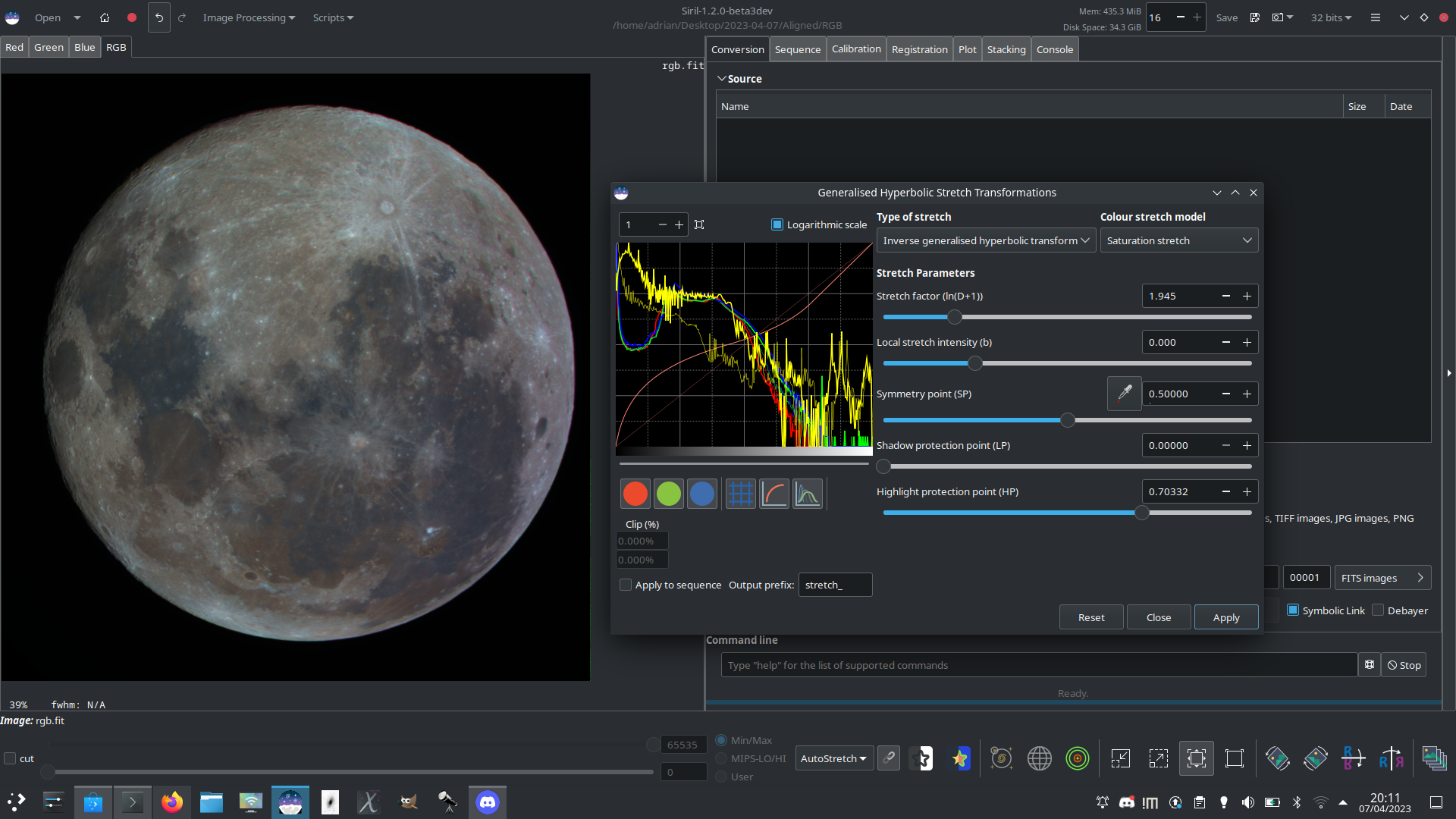
remapping image saturation: the GHS transforms can be applied to the image
saturation channel by selecting the Saturation option from the Color stretch
model combo box. When this mode is selected the pre- and post- stretch
saturation histograms will be shown in yellow. All the GHS options are available
and this mode can provide highly targeted adjustment of the image saturation
channel. A simple method of increasing the saturation in relatively
unsaturated regions while preventing oversaturation is to use an Inverse
generalised hyperbolic transform stretch with SP set to around 0.5, and
HP brought down low enough to flatten the upper end of the saturation
histogram.
In order to control partially-clipped highlights, the GHS tool makes available the
same range of clipping modes as the asinh stretch. Details can be found here.
The image above shows how applying the GHS tool to the saturation channel gives
an easy way of strongly enhancing saturation in a low-saturation image while
still retaining control of the upper end of the saturation histogram, here used
to create a 'Mineral Moon' image highlighting the differing mineral composition
of different regions of the lunar surface.
Generalised hyperbolic stretch based on the work of the ghsastro.co.uk team.
The argument -D= defines the strength of the stretch, between 0 and 10. This is the only mandatory argument. The following optional arguments further tailor the stretch:
B defines the intensity of the stretch near the focal point, between -5 and 15;
LP defines a shadow preserving range between 0 and SP where the stretch will be linear, preserving shadow detail;
SP defines the symmetry point of the stretch, between 0 and 1, which is the point at which the stretch will be most intense;
HP defines a region between HP and 1 where the stretch is linear, preserving highlight details and preventing star bloat.
If omitted B, LP and SP default to 0.0 ad HP defaults to 1.0.
An optional argument (either -human, -even or -independent) can be passed to select either human-weighted or even-weighted luminance or independent colour channels for colour stretches. The argument is ignored for mono images. Alternatively, the argument -sat specifies that the stretch is performed on image saturation - the image must be color and all channels must be selected for this to work.
Optionally the parameter [channels] may be used to specify the channels to apply the stretch to: this may be R, G, B, RG, RB or GB. The default is all channels. The clip mode can be set using the argument -clipmode=: values clip, rescale, rgbblend or globalrescale are accepted and the default is rgbblend. This command is mask-aware and will obey the mask if and only if the -mask flag is provided
Inverts a generalised hyperbolic stretch. It provides the inverse transformation of GHT, if provided with the same parameters, undoes a GHT command, possibly returning to a linear image. It can also work the same way as GHT but for images in negative. This command is mask-aware and will obey the mask if and only if the -mask flag is provided
Modified arcsinh stretch based on the work of the ghsastro.co.uk team.
The argument -D= defines the strength of the stretch, between 0 and 10. This is the only mandatory argument. The following optional arguments further tailor the stretch:
LP defines a shadow preserving range between 0 and SP where the stretch will be linear, preserving shadow detail;
SP defines the symmetry point of the stretch, between 0 and 1, which is the point at which the stretch will be most intense;
HP defines a region between HP and 1 where the stretch is linear, preserving highlight details and preventing star bloat.
If omitted LP and SP default to 0.0 ad HP defaults to 1.0.
An optional argument (either -human, -even or -independent) can be passed to select either human-weighted or even-weighted luminance or independent colour channels for colour stretches. The argument is ignored for mono images. Alternatively, the argument -sat specifies that the stretch is performed on image saturation - the image must be color and all channels must be selected for this to work.
Optionally the parameter [channels] may be used to specify the channels to apply the stretch to: this may be R, G, B, RG, RB or GB. The default is all channels. The clip mode can be set using the argument -clipmode=: values clip, rescale, rgbblend or globalrescale are accepted and the default is rgbblend. This command is mask-aware and will obey the mask if and only if the -mask flag is provided
Inverts a modified arcsinh stretch. It provides the inverse transformation of MODASINH, if provided with the same parameters, undoes a MODASINH command, possibly returning to a linear image. It can also work the same way as MODASINH but for images in negative. This command is mask-aware and will obey the mask if and only if the -mask flag is provided
Stretches the image linearly to a new black point BP.
The argument [channels] may optionally be used to specify the channels to apply the stretch to: this may be R, G, B, RG, RB or GB. The default is all channels.
Optionally the parameter -sat may be used to apply the linear stretch to the image saturation channel. This argument only works if all channels are selected. The clip mode can be set using the argument -clipmode=: values clip, rescale, rgbblend or globalrescale are accepted and the default is rgbblend
Applying transformation to the sequence
This transformation can easily be applied to a sequence. You just have to
define the transformation on the loaded image (with a sequence already loaded),
then check the Apply to sequence button and define the output prefix of
the new sequence (stretch_ by default). All of the commands have a sequence
processing form too. Each sequence stretching command starts with seq and the
first argument must be the sequence name, but they are otherwise the same.
Same command as GHT but the sequence must be specified as the first argument. In addition, the optional argument -prefix= can be used to set a custom prefix
Same command as INVGHT but the sequence must be specified as the first argument. In addition, the optional argument -prefix= can be used to set a custom prefix
Same command as MODASINH but the sequence must be specified as the first argument. In addition, the optional argument -prefix= can be used to set a custom prefix
Same command as INVMODASINH but the sequence must be specified as the first argument. In addition, the optional argument -prefix= can be used to set a custom prefix
Same command as LINSTRETCH but the sequence must be specified as the first argument. In addition, the optional argument -prefix= can be used to set a custom prefix
Curves Transformation is a highly versatile tool used to adjust the contrast, the
brightness and the colors of an image by modifying the pixel values according to
custom-defined curves. This allows for precise control over the image's stretch.
The tool is built on the VeraLux curve engine, ported into the Siril core from the
VeraLux_Curves.py script (see the list of Python scripts). On
top of the classical per-channel curves, it provides curves acting on perceptual
quantities (luminance, chroma and saturation), a luminance range mask that
restricts where a curve is applied, and a non-destructive workflow based on
stages.
A curve is defined by a series of points, each of which can be moved to shape it.
The curve is interpolated between these points, and the pixel values are
transformed based on it. This allows for a wide range of transformations to be
applied to the image, from simple linear stretches to complex non-linear
adjustments.
a left-click on an empty area of the graph adds a point, which can then be
dragged around. A curve holds at most 100 points.
a left-click on an existing point selects it, so that it can be dragged or
edited numerically.
a right-click on a point removes it. A curve always keeps at least two
points, so the last two cannot be removed.
The ID, X and Y fields below the graph give
the index and the exact coordinates of the selected point, and can also be used
to type them in. The arrows next to the ID field walk through the
points of the curve.
The histogram of the image is drawn behind the curve, so that the effect of the
transformation can be judged against the tonal distribution of the image. It
follows the selected channel: the red, green and blue histograms are shown for
the RGB/K, R, G and B channels, while the L, C and S channels display the
histogram of the corresponding quantity.
The Logarithmic scale checkbox displays the histogram with a
logarithmic scale, which is useful for images with a wide dynamic range as it
makes the shadows and the highlights more readable. It does not affect the
display of the transfer curve itself. The zoom spin button stretches the graph
horizontally inside its scrolled area, which helps to place points precisely in
the deep shadows, and the button next to it resets the zoom to 1. The grid button
toggles the grid overlay.
The Clip (%) fields report the percentage of pixels that the current
transformation pushes to pure black (left field) and to pure white (right field).
The pipette button turns the cursor into a picking tool: clicking anywhere on the
image draws a vertical marker on the graph at the value of the clicked pixel,
showing where on the curve a given part of the image lies. The value is read in
the space of the currently selected channel, and always from the image as it was
before the curves were applied, so that the marker follows the horizontal axis of
the graph even while the preview is on.
Three interpolation algorithms are available in the Curves Transformation dialog:
linear, cubic spline and Akima spline, the latter being the default.
Theory
Linear interpolation is a simple interpolation that connects the points with straight lines.
For each pair of points, the slope of the line connecting the points is calculated:
Cubic spline curves are more complex curves that are defined by a series of control
points. For pixel value \(x\) between two control points \(x_i\) and \(x_{i+1}\),
the curve is defined by the following equation:
For \(x_i < x < x_{i+1}\), the coefficients \(a_i, b_i, c_i\), and \(d_i\) are calculated by
solving a system of equations derived from the conditions of continuity and
smoothness at each internal point. These conditions are:
The spline must be continuous at each internal point,
The first derivative of the spline must be continuous at each internal point,
The second derivative of the spline must be continuous at each internal point
Since Curves Transformation uses natural cubic splines, the second derivative at both endpoints is 0.
Akima splines are piecewise cubic as well, but their coefficients are
derived from local slopes only, instead of a global system of equations.
Noting \(m_i = (y_{i+1} - y_i) / (x_{i+1} - x_i)\) the slope of the
segment between two consecutive points, the slope assigned to point
\(i\) is:
and the curve on each interval is the cubic that matches the two end points
and these two slopes. The two missing slopes at each end of the curve are
extrapolated from their neighbours, and the average of the two neighbouring
slopes is used when the denominator vanishes. Because only the closest
neighbours are involved, a point moved in one part of the curve does not
ripple through the whole transfer function, and Akima splines do not
overshoot around abrupt slope changes the way natural cubic splines do. This
is what makes them a safer default for image data. The construction requires
at least three points, so a two-point curve falls back to the straight line
joining them.
The row of buttons on the right of the graph selects which curve is being
edited. Each channel keeps its own set of points and its own range masking
settings, and they are all applied in a single pass when the transformation runs.
Channel
Quantity the curve is applied to
RGB/K
The master curve: the same transfer function is applied to the three
channels of a color image, or to the single channel of a monochrome image.
R, G, B
The red, green and blue channels, each independently. Typically used to
correct a color cast that survived color calibration.
L
The CIE \(L^*\) lightness, normalized to \([0, 1]\) by dividing it
by 100. The transformation is done in the CIE Lab space and the chromatic
components \(a^*\) and \(b^*\) are left untouched, so brightness is
modified without shifting the colors.
C
The chroma of the CIE Lab space, \(C = \sqrt{a^{*2} + b^{*2}}\),
normalized by dividing it by 128. Both \(a^*\) and \(b^*\) are
scaled by the same factor, so the hue and the lightness are preserved while
the colorfulness is increased or reduced.
S
The saturation of the HSV space. Compared to the C curve, it acts closer to
the way display software saturates an image, and is more aggressive on
already colorful areas.
The curves are always applied in the following order: RGB/K, then R, G and B,
then L, then S and finally C. Each of them sees the pixel as the previous ones
left it, which matters when several channels are used at the same time.
Warning
The R, G, B, L, C and S channels are only meaningful on color images and are
therefore disabled when a monochrome image is loaded. Only the master RGB/K
curve remains available in that case.
Tip
Increasing the saturation of an image often brightens it as a side effect, and
stretching its luminance often washes the colors out. Combining a L curve and a
C or S curve in a single Curves Transformation lets you compensate one with the
other while judging the result on a single preview.
By default a curve applies to every pixel of the image. Enabling
Enable Range Masking restricts it to a range of luminance, so that,
for instance, saturation can be boosted in the bright parts of a nebula without
touching the noisy background, or the background can be darkened without
flattening the object.
Three sliders, all expressed in percent, define the mask of the current channel:
Min and Max bound the luminance range the curve applies
to. Their default values, 0 and 100, cover the whole image.
Feather controls how progressively the curve fades out at both ends
of the range, 25% by default. A value of 0 gives a hard cut, which usually
shows as visible edges in the result, while larger values give a smoother, more
natural transition.
The Show mask checkbox, only available once range masking is enabled,
replaces the preview by the mask itself, rendered as a grayscale image: white
means the curve is fully applied, black means the pixel is left untouched, and
the grays in between show the feathered transition. This is the fastest way to
check that a range actually selects the region you had in mind. Unchecking it
brings the regular preview back.
Theory
The mask is computed per pixel from the mean of its three channels,
\(Y = (R + G + B) / 3\), taken as the pixel stands when the channel is
applied. With a feather \(f > 0\) the roll-off is a pure sigmoid
\(\sigma(x) = 1 / (1 + e^{-x})\) of steepness \(k = 2.5\):
where the first term is dropped when \(Y_{min} = 0\) and the second when
\(Y_{max} = 1\). When \(f = 0\) the mask is simply 1 inside
\([Y_{min}, Y_{max}]\) and 0 outside. The output of the channel is then
the blend:
The mask is strictly pointwise: no spatial blur is involved, which preserves
the pixel-to-pixel fidelity of the data and cannot create halos around bright
objects.
Complex adjustments are rarely obtained with a single set of curves. Rather than
closing and reopening the dialog to chain several transformations, the curves can
be committed as stages, without leaving the tool.
Apply Stage bakes the curves currently defined into the working
image and resets every channel to the identity curve, ready for the next
adjustment. The image displayed is updated, but nothing is written to the undo
history yet.
↩ Stage removes the last committed stage. The image is rebuilt from
the state it had when the dialog was opened and the remaining stages are
replayed on it, so the operation is exact and can be repeated until the stack is
empty. The button is insensitive when there is no stage to undo.
Apply commits everything, the stages and the curves currently being
edited, as a single undo entry.
Tip
Because a stage is only baked into the working image, and not into the undo
history, the whole sequence of stages is undone in one step from the main
window afterwards. This keeps the undo history readable while allowing an
arbitrary number of successive adjustments.
Reset channel restores the identity curve and the default masking
settings of the selected channel only, while Reset all does the same
for all the channels at once and resets the zoom. Neither of them touches the
stages that have already been committed.
Some common uses of the Curves Transformation tool include:
"S" curve: This curve is used to increase the contrast of an image. By increasing the
slope of the curve in the middle of the histogram, the contrast is increased.
BP & WP adjustments: The black point (BP) and white point (WP) of an image can be adjusted
by moving the first and last control points of the curve. This allows for the shadows and
highlights of the image to be adjusted independently.
An example of adjusting the black point and white point of an image
Targeted adjustments: By adding control points at specific locations in the histogram, targeted
adjustments can be made to the image. For example, the shadows can be darkened without affecting
other parts of the image.
Selective color boost: select the C channel, raise the middle of the curve,
then enable range masking and set Min just above the level of the
background. The colors of the object are reinforced while the background, where
chroma is mostly noise, is left alone.
Tip
The Curves Transformation tool is best used on an image that has already been stretched to
some extent. This allows for more precise control over the image's contrast and brightness.
Tip
If a ROI is set, the histogram preview will not update to show the impact
of the stretch on the ROI. This is because that behaviour could be misleading:
if the ROI is not typical of the image overall, adjusting the ROI histogram
to a suitable level would result in a badly adjusted histogram for the
overall image and potentially a burned-out or excessively dark look to the
result. When in ROI mode the stretch parameters should be adjusted by eye.
If it is desired to check the histogram for the stretch as applied to the
image as a whole, the ROI should be cleared.
This transformation can easily be applied to a sequence. All you have to do is
define the transformation on the loaded image while a sequence is loaded
and check the Apply to sequence button. Similarly to other stretching
tools, you can define the output prefix of the new sequence (curve_ by default).
All the channels and their range masking settings are applied to each image of
the sequence, but the stages are not: commit them with Apply on the
loaded image beforehand if you need them.
 allows you to apply the same transformation as the autostretch algorithm. It
is rarely advisable to use this button as is. Adjustments are usually
necessary to avoid losing information.
allows you to apply the same transformation as the autostretch algorithm. It
is rarely advisable to use this button as is. Adjustments are usually
necessary to avoid losing information.