Intensity Profiling

Profile button icon

Siril has an intensity profiling mode. The user selects a line between two points and Siril will generate a graph of the pixel values between them. This has several uses. It can be used to inspect the intensity profile of an individual star, it can be used to profile a whole galaxy, or it can be used to make spectrograms if you have a diffraction grating filter such as the Star Analyzer SA-100 or a true spectrograph.

Basic Intensity Profile

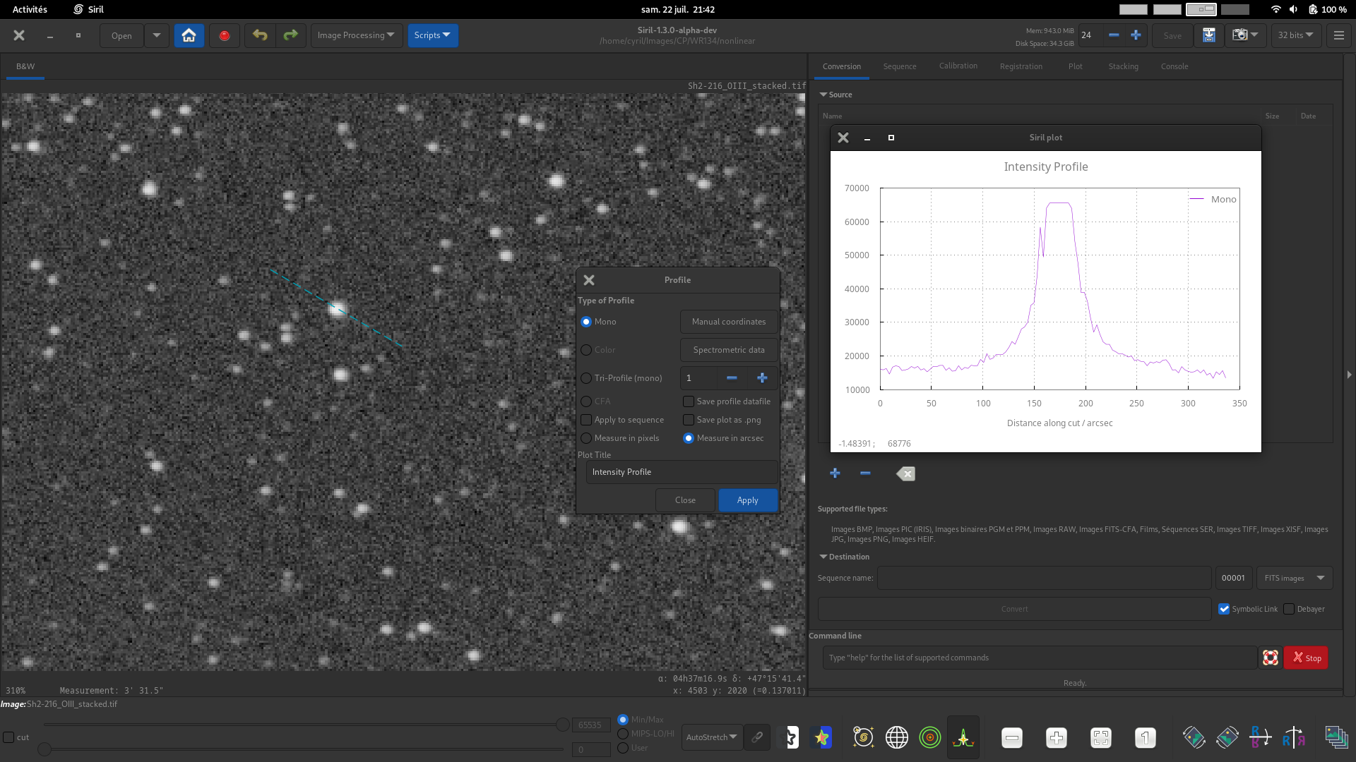
To make a basic intensity profile of a star or other object, select the Profile button in the bottom toolbar. This puts Siril into profiling mode and opens a small dialog.

Profile button icon

You can now click and drag on the main image display to set the start and finish points of the line you wish to profile. If you hold down the Shift key while dragging the line, it will snap to be either horizontal or vertical.

Tip

When the profile line is exactly horizontal or exactly vertical, exact pixel values can be used directly from the image. When the profile line is neither horizontal nor vertical, the points to be plotted do not fall exactly on a pixel and bilinearly interpolated pixel values are therefore used.

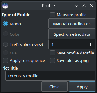
A custom title for your plot can be entered in the control at the bottom of the dialog.

Tip

When processing a sequence, it is possible to have the custom title display the image number and total by adding () to the end of the title. For example entering Solar Spectra () as the title for a 5 image sequence will generate titles Solar Spectra (1 / 5), Solar Spectra (2 / 5) etc. The brackets are ignored and removed if processing a single image.

Types of Profile

Use the radio buttons to select the type of profile you want. (Click on the example images below to see them full size.)

  • Mono profile. For mono or color images, generate a luminance profile between two points. This mode can be used with spectrometric data.

Profile button icon

Tip

If a color image is loaded but the mono profiling mode is selected, the profile will be made according to the viewport. The R, G and B viewports provide mono profiles of their respective channel and the RGB viewport provides a luminance profile weighting all 3 channels equally.

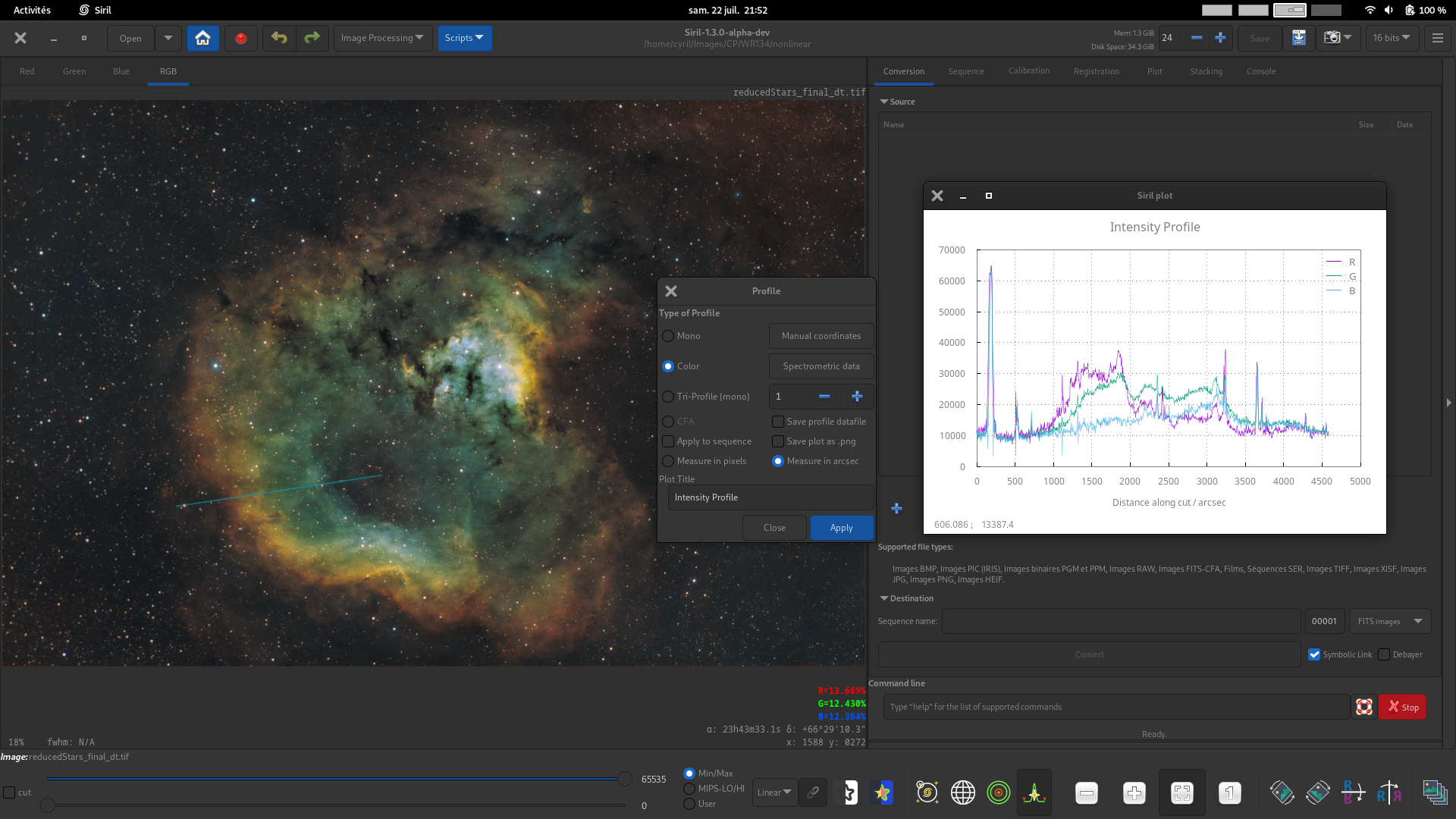
  • Color profile. For color images, generate three profiles for the R, G and B pixel values between two points. This mode can be used with spectrometric data.

Profile button icon
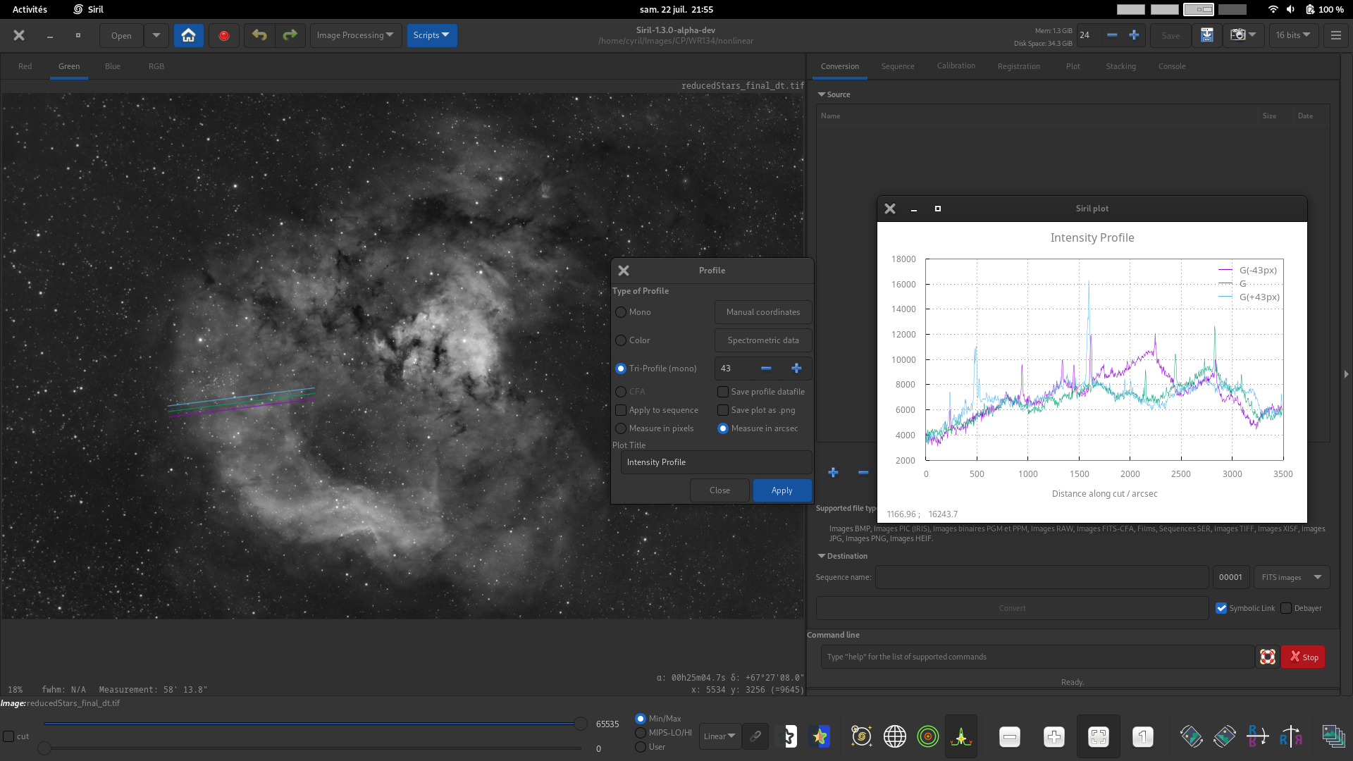
  • Tri-profile (mono). For mono or color images, generate three parallel equispaced luminance profiles between two points. The spacing between the 3 profiles can be set using the spin button.

Profile button icon
  • CFA. For images with a Bayer pattern only, generate four profiles for the four CFA subchannels between two points. This can be particuarly useful for inspecting the profile of Bayer patterned flats or other Bayer pattern images before they are debayered.

Profile button icon

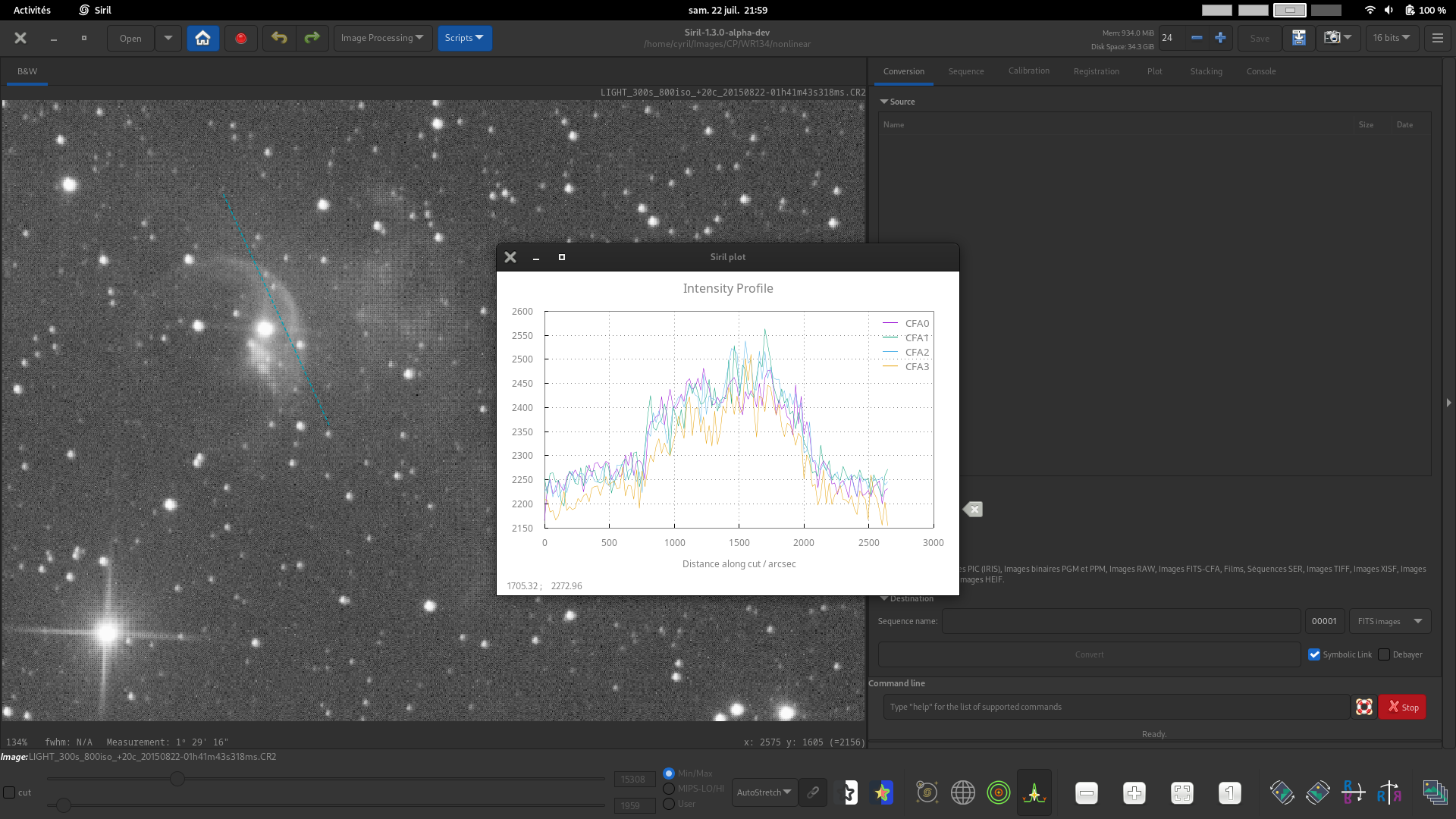
This image demonstrates use of the Custom Title control to set a custom title for the plot.

Note

Spectrometric data options are mutually exclusive with tri-profiling and CFA profiling modes: tri-profiling and CFA profiling will ignore any wavenumber data provided and the profile width option.

Click Apply to generate your profile.

Precise Coordinate Entry

In order to make it easy to input coordinates precisely and repeatably, a manual entry method is provided. Click the Manual Coordinates button and you can enter the X and Y coordinates of the start and end points of the profile line. If a profile line is already drawn but one point is not quite in the place you want it, you can use this popup dialog to fine tune the placement of the endpoints.

If you wish to set an endpoint exactly to the position of a star, make a rectangular selection around the star and click the relevant star button to the right of the dialog. This is especially useful when conducting spectrography with a diffraction grating filter as it aids in drawing the profile exactly through the centre of the diffracted spectrum.

Tip

When using this method for spectrography, the star whose spectrum is being graphed must be selected as the start point, not the end point, otherwise the wavenumber axis will end up being backwards.

Note

When using the CFA mode, coordinates are given in the input image. However each CFA channel is half the width and half the height. The x axis in the CFA mode plot is measured in pixels in the CFA subchannel, i.e. it will span half the number of pixels that it does in the input image.

Measurement

The intensity profile line can be used as a measuring tool in two ways:

  • Checking the Measure profile checkbox will measure all profile lines dragged with the mouse, similarly to the Ctrl + Shift + Drag quick measurement function.

  • In the Coordinates dialog there is a Measure button. This provides the same measurement function but allows you to set the endpoints exactly, and then measure the profile line on demand. By selecting stars, minor planets or comet nuclei as end points as described above, measurements between two celestial bodies can be made very precisely (with sub-pixel precision).

Profile button icon

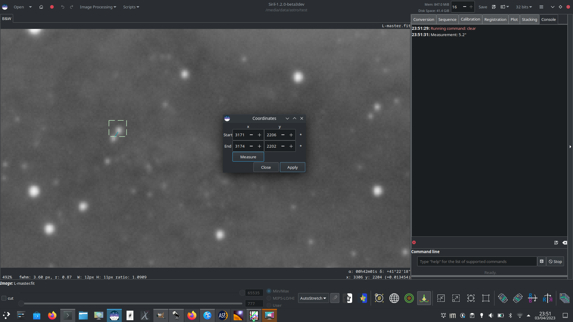
Here, two close stars have been selected and set as the endpoints and the separation between them measured as 5.2 arcsec. This could be used to study close binaries or to triangulate the position of a minor planet.

Note

Siril's measurement function makes the small angle approximation for the angular separation \(\theta\). The most significant error term is proportional to \(\theta^3\) and is less than 1% for measurements up to 10°: it is therefore valid for most astrometric uses, but will become inaccurate for large measurements across ultra-wide field images. A warning will be written to the log for measurements over 10°.

Spectrography

You may have a spectrograph or diffraction grating filter. In that case you can use additional features of the profiling mode to produce a spectrogram. Click on the Spectrometric data button to input data relating to spectral measurements.

In order to reduce noise, a cut width can be specified. If this is greater than 1 an average value of multiple pixels perpendicular to the cut line will be used at each point instead of a single value. A greater width will reduce noise more, but if using a diffraction grating the spectrum of a star is fairly narrow so there is only so wide the profile can be made before extending outside the region of the image where the spectral data is.

To calibrate the wavenumber axis it is possible to select two points on the graph with known wavenumbers or wavelengths, for example known absorption lines. To do so, first click the Pick point 1 button, and click on the image at the location corresponding to the first known wavenumber. The x and y coordinates chosen will snap to the closest point on the cut line. If you click on the wrong place, simply click the button again and reselect the point. Repeat this process for the second known wavenumber or wavelength, this time using the Pick point 2 button.

You can also choose whether to plot your spectrogram with an x axis showing wavelength (the default) or wavenumber using the combo box.

Note

The axis calibration relies on the small axis approximation, i.e. the distance along the x axis is proportional to wavelength. This comes from the diffraction equation \(d \sin(\theta) = m \lambda\). This gives the distance diffracted along an x axis perpendicular to the grating of \(x = D \tan\left(\arcsin\left(\frac{m \lambda}{d}\right)\right)\) and the x axis error is less than 1% as long as the angle diffracted is less than 9 degrees. This is true for many diffraction gratings, for example the Star Analyser SA-100 has a line spacing of 100 lines / mm. For hydrogen alpha emissions with a wavelength of 656nm, this gives a first order diffraction angle of 0.125 degrees.

Profile button icon

Once you are happy with your choices here, click Apply to return to the main profiling dialog. You can now click Apply to generate your spectrogram.

Profile button icon

Here is a solar FeH spectrum captured using the THEMIS telescope, averaged over 15 pixels per column to improve SNR and with the wavenumber axis labelled using the Spectrometric Data popup.

Profile button icon

As an example, here are the hydrogen lines of the Balmer series taken through a diffraction grating. Two lines were used (\(\text{H}_\alpha\) and \(\text{H}_\beta\)) to calibrate the spectrum.

Note

The wavenumber, as used in spectroscopy and most chemistry fields, is defined as the number of wavelengths per unit distance, typically centimeters (cm \(^{−1}\)):

(1)\[{\displaystyle {\tilde {\nu }}\;=\;{\frac {1}{\lambda }},}\]

where \(\lambda\) is the wavelength. It is sometimes called the spectroscopic wavenumber. It equals the spatial frequency.

Siril Plot Tool

The profiling feature uses Siril internal plotting tool to display the different profiles. With the *.dat files produced, you can still use any plotting tool of your liking to explore the underlying data.

A right-click anywhere in the plotting surface will pop-up a contextual menu to:

  • Show/hide grids and legend

  • Export current view to clipboard, *.png or *.svg

  • Save underlying data to a *.dat file

Siril plot menu

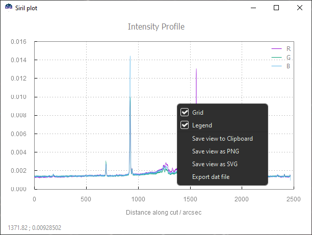
Siril plot contextual menu

Note that all exports account for the current zoom/pan while saving to dat will export unfiltered data.

The following GUI interactions are avalaible:

  • Click + Drag to draw a selection. The zoom is set to the selected zone when the mouse is released.

  • Ctrl + Drag to pan the current view.

  • Ctrl + Scroll to zoom in/out.

  • Double-click to reset to the default position/zoom.

Commands

Siril command line

profile -from=x,y -to=x,y [-tri] [-cfa] [-arcsec] { [-savedat] | [-filename=] } [-layer=] [-width=] [-spacing=] [ {-xaxis=wavelength | -xaxis=wavenumber } ] [ {-wavenumber1= | -wavelength1=} -wn1at=x,y {-wavenumber2= | -wavelength2=} -wn2at=x,y] ["-title=My Plot"]
Generates an intensity profile plot between 2 points in the image, also known as a cut. The arguments may be provided in any order. The arguments -to=x,y and -from=x,y are mandatory.

The argument -layer={red | green | blue | lum | col} specifies which channel (or luminance or colour) to plot if the image is color. This can be used in conjunction with spectrometric options. It may also be used with the -tri option, which generates 3 parallel equispaced profiles each separated by -spacing= pixels, but note that for tri profiles the col option will be treated the same as lum.

The option -cfa selects CFA mode, which generates 4 profiles: 1 for each CFA channel in a Bayer patterned image. This option cannot be used with color images or mono images with no Bayer pattern, and cannot be used at the same time as the -tri option.

The option -arcsec causes the x axis to display distance in arcsec, if the necessary metadata is available. This option is overridden if spectrometric options are provided. If not provided or if metadata is not available, distance will be shown in pixel units.

The argument -savedat will cause the data files to be saved: the filename will be written to the log. Alternatively the argument -filename= can be used to specify a filename to write the data file to. (The -filename= option implies -savedat.)

Spectrometric Options

If spectrometric options are provided, all of the following must be provided: -wavenumber1= / -wavelength1= and -wavenumber2= / -wavelength2= specify 2 wavenumbers in cm-1 / wavelengths in nm, and -wn1=x,y and -wn2=x,y specify points in the image corresponding to those wavenumbers. As a convenience, -wavelength1= and -wavelength2= may be used instead to provide wavelengths in nm. The following optional spectrometric arguments may be provided: -width=, which specifies how many pixels should be averaged perpendicular to the profile line, and one of -xaxis=wavelength or -xaxis=wavenumber, which set the units for the x axis (the default is wavelength).

The argument "-title=My Title" sets a custom title "My Title"

Siril command line

seqprofile sequence -from=x,y -to=x,y [-tri] [-cfa] [-arcsec] [-savedat] [-layer=] [-width=] [-spacing=] [ {-xaxis=wavelength | -xaxis=wavenumber } ] [{-wavenumber1= | -wavelength1=} -wn1at=x,y {-wavenumber2= | -wavelength2=} -wn2at=x,y] ["-title=My Plot"]
Generates an intensity profile plot between 2 points in each image in the sequence. After the mandatory first argument stating the sequence to process, the other arguments are the same as for the profile command. If processing a sequence and it is desired to have the current image number and total number of images displayed in the format "My Sequence (1 / 5)", the given title should end with () (e.g. "My Sequence ()" and the numbers will be populated automatically)