Principles

Photometry is the science of the measurement of light. It aims to measure the flux or intensity of light radiated by astronomical objects. In Siril, photometry can be used to analyze the light curve of variable stars, transits of exoplanets or occultations of stars, or to calibrate colors in RGB images.

Aperture photometry is the method used. Its basic principle is to sum-up the observed flux in a given radius from the center of an object, then subtract the total contribution of the sky background in the same region (calculated in the ring between the inner and outer radii, excluding the deviant pixels), leaving only the flux of the object to calculate an instrumental magnitude. This is illustrated in the following figure.

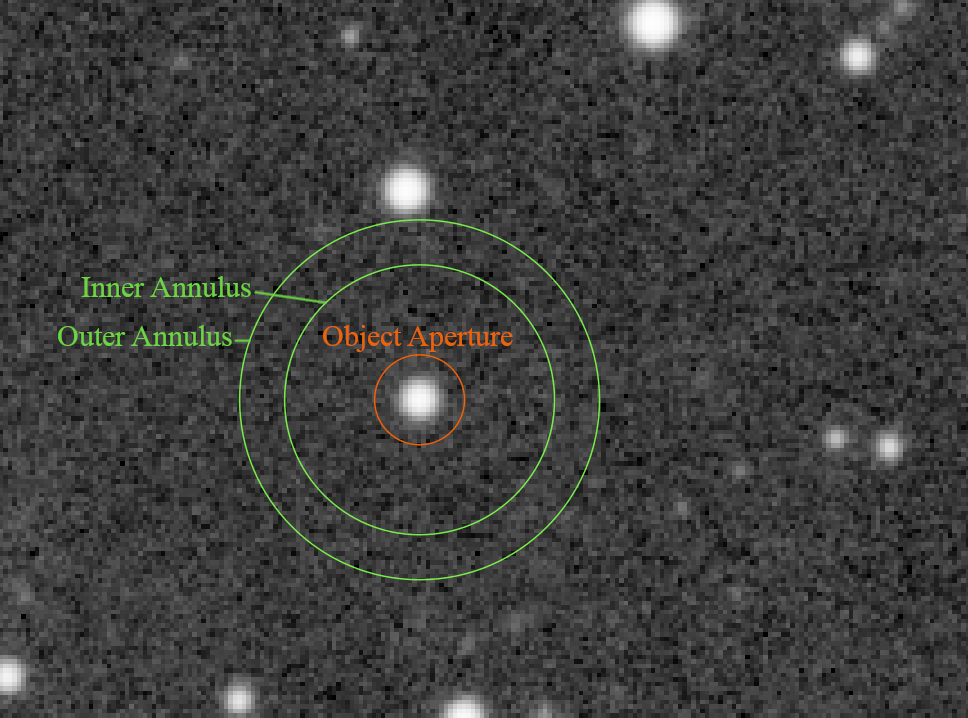
Circles of the aperture photometry

The values of these settings can be changed in the Photometry section of preferences or using the setphot command. The aperture must contain all pixels of the object to measure, the annulus should by opposition not contain any of its pixels. By default, the aperture is adjusted for a target using twice the PSF's FWHM, but the annulus size is fixed. These values should be adjusted for a given sampling, and checked with care.

Note

The following text is a truncated and modified copy of the excellent MuniPack software documentation, from David Motl and released under the GNU Free Documentation License, whose sources are available here.

Measuring magnitude of an object

The sum S of pixels in a small area A around an object is a sum of the object's net intensity I plus background intensity \(B\cdot A\):

(1)\[ S = I + B\cdot A\]

The values of S and B are derived from the source frame, the area A is determined as the area of circle of radius r, where r is the size of the aperture in pixels. It is then easy to compute the net intensity I of an object in ADU:

(2)\[ I = S - B\cdot A\]

Supposing that the net intensity I is proportional to the observed flux F, we can derive the apparent magnitude m of the object, utilizing the Pogson's law:

(3)\[ m = -2.5 \log_{10}\left(\frac{I}{I_0}\right)\]

Estimating the measurement error

Once we have derived the raw instrumental brightness of an object, we will try to estimate its standard error. First of all, we will recall a few general rules that apply to the standard error and its propagation. This is a general rule for error propagation through a function f of uncertain value X:

(4)\[ \operatorname{Var}(f(X)) = \left(\frac{df}{dx}\right)^2 \operatorname{Var}(X)\]

Using this general rule, we derive two laws of error propagation. In the first case, the uncertain value X is multiplied by a constant a and shifted by a constant offset b. This law can also be used in the case where only a multiplication or only an offset occurs.

(5)\[ \operatorname{Var}(aX + b) = a^2 \operatorname{Var}(X)\]

The second law defines the error of a logarithm of uncertain value X:

(6)\[ \operatorname{Var}(\log(\pm bX)) = \frac{\operatorname{Var}(X)}{\bar{X}^2}\]

Please note, that the log function here is the natural logarithm, while the Pogson's formula (see above) incorporates the base-10 logarithm. The following equation helps us to deal with this difference:

(7)\[ \log_b(x) = \frac{\log_k(x)}{\log_k(b)}\]

Putting these two equations together we get:

(8)\[ \operatorname{Var}(\log_{10}(\pm bX)) = \frac{\operatorname{Var}(X)}{\bar{X}^2\,\log(10)^2}\]

If we have two uncorrelated uncertain variables X and Y, the variance of their sum is the sum of their variances, this equation is known as Bienaymé formula.

(9)\[ \operatorname{Var}(X + Y) = \operatorname{Var}(X) + \operatorname{Var}(Y)\]

From this formula, we can also derive the standard error of a sample mean. If we have N observations of random variable X with sample-based estimate of the standard error of the population s, then the standard error of a sample mean estimate of the population mean is

(10)\[ SE_{\bar{X}} = \frac{s}{\sqrt{N}}\]

Armed with this knowledge, we can start thinking about the estimation of standard error of object brightness. We will consider the following three sources of uncertainty: (1) random noise inside the star aperture that includes the thermal noise of the detector, read-out noise of the signal amplifier and the analog-to-digital converter, (2) Poisson statistics of counting of discreet events (photons incident on a detector) that occur during a fixed period of time and (3) the error of estimation of mean sky level.

For the estimation of mean sky level, we have used the robust mean algorithm. It allows to estimate its sample variance \(\sigma_{pxl}^2\). This is a pixel-based variance and because we have summed together A pixels in the star aperture, the Bienaymé formula applies, the sum S is a sum of A uncorrelated random variables, each of which has variance \(\sigma_{pxl}^2\). For the variance of the first source of error we get:

(11)\[ \sigma_1^2 = A\,\sigma_{pxl}^2\]

where A is a number of pixels in the star aperture.

From Poisson statistics we can derive a variance that occur due to counting of discreet events, photons incident on a detector, that occur during a fixed period of time, the exposure. We will again need to use the gain p of the detector to convert a intensity in ADU to a number of photons. If the measured net intensity of an object is I we compute the mean number of photons \(\lambda\) as

(12)\[\lambda = I\,p\]

Note

The value of the gain p of the detector can be changed in the Photometry section of Siril's preferences

Then, the variance of intensity due to Poisson statistics is equal to its mean value.

(13)\[ \sigma_{ph}^2 = \operatorname{Var}(\operatorname{Pois}(\lambda)) = \lambda = I\,p\]

The variance is in photons, we have to convert it back to ADU to get the variance in units \(ADU^2\).

(14)\[ \sigma_2^2 = \frac{\sigma_{ph}^2}{p^2} = \frac{I\,p}{p^2} = \frac{I}{p}\]

We have derived the sky level as a sample mean of pixel population in the sky annulus. Because each pixel in the annulus has variance \(\sigma_{pxl}^2\), the variance of sample mean is

(15)\[ s_{sky}^2 = \frac{\sigma_{pxl}^2}{n_{sky}}\]

where \(n_{sky}\) is the number of pixels in sky annulus.

From equation (9) we compute the variance of object's intensity as

(16)\[ \sigma_{ADU}^2 = \sigma_1^2 + \sigma_2^2 + A^2\,s_{sky}^2\]

Note, that in equation (2) the sky level is multiplied by A, so we have to multiply its variance by \(A^2\) - see the equation (16). Now, we use the law of error propagation for the logarithm adopted to match the formula of the Pogson's law.

(17)\[ \sigma_{mag}^2 = \left(\frac{-2.5}{I\,\log(10)}\right)^2\,\sigma_{ADU}^2\]

Putting equations (17) and (16) together, we can derive the standard error of the object's brightness in magnitudes as

(18)\[ \sigma_{mag} = \frac{1.08574}{I}\,\sqrt{\sigma_{ADU}^2}\]