Deconvolution
Deconvolution is a mathematical tool to compensate for blurring or distorting effects in an image. The true scene is not what is recorded on your sensor - you record an estimate of the true scene convolved by a PSF (in mathematical terms, the "blurring PSF" that represents atmospheric distortion, physical properties of your telescope, motion blur and so on, degrading your estimate). Deconvolution can, to an extent, reverse this image degradation. However, it is important to say up front that deconvolution is what mathematicians call an ill-posed problem (like most inverse problems). Ill-posed means that either a solution may not exist, if a solution does exist it may not be unique, and it may not have continuous dependence on the data. Essentially it means deconvolution is, even theoretically, really hard and there are no guarantees it will work.
All this is made even harder when we don't know exactly what the PSF is that we're trying to remove. In astronomy we can in theory get an idea of the PSF by the effect of blurring on the point sources (stars) that we are imaging. However sometimes the true PSF isn't constant across the image, sometimes other factors such as star saturation prevent the star PSF being an entirely accurate estimate of the PSF, and sometimes (for example lunar imaging) there are no stars.
Siril aims to provide a flexible approach to deconvolution. There are several options for defining or estimating the PSF, and several deconvolution algorithms to choose from for the final stage of deconvolution once the PSF is defined.
Example of deconvolution on star field.
Deconvolution is accessed through the Image Processing menu or using Siril commands.
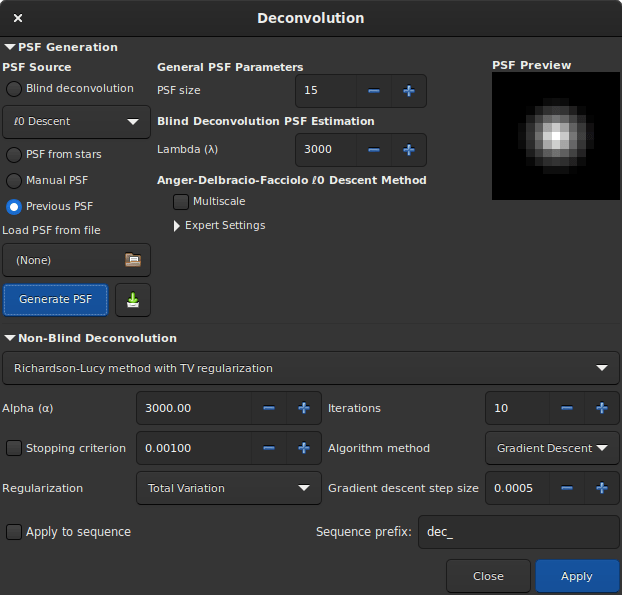
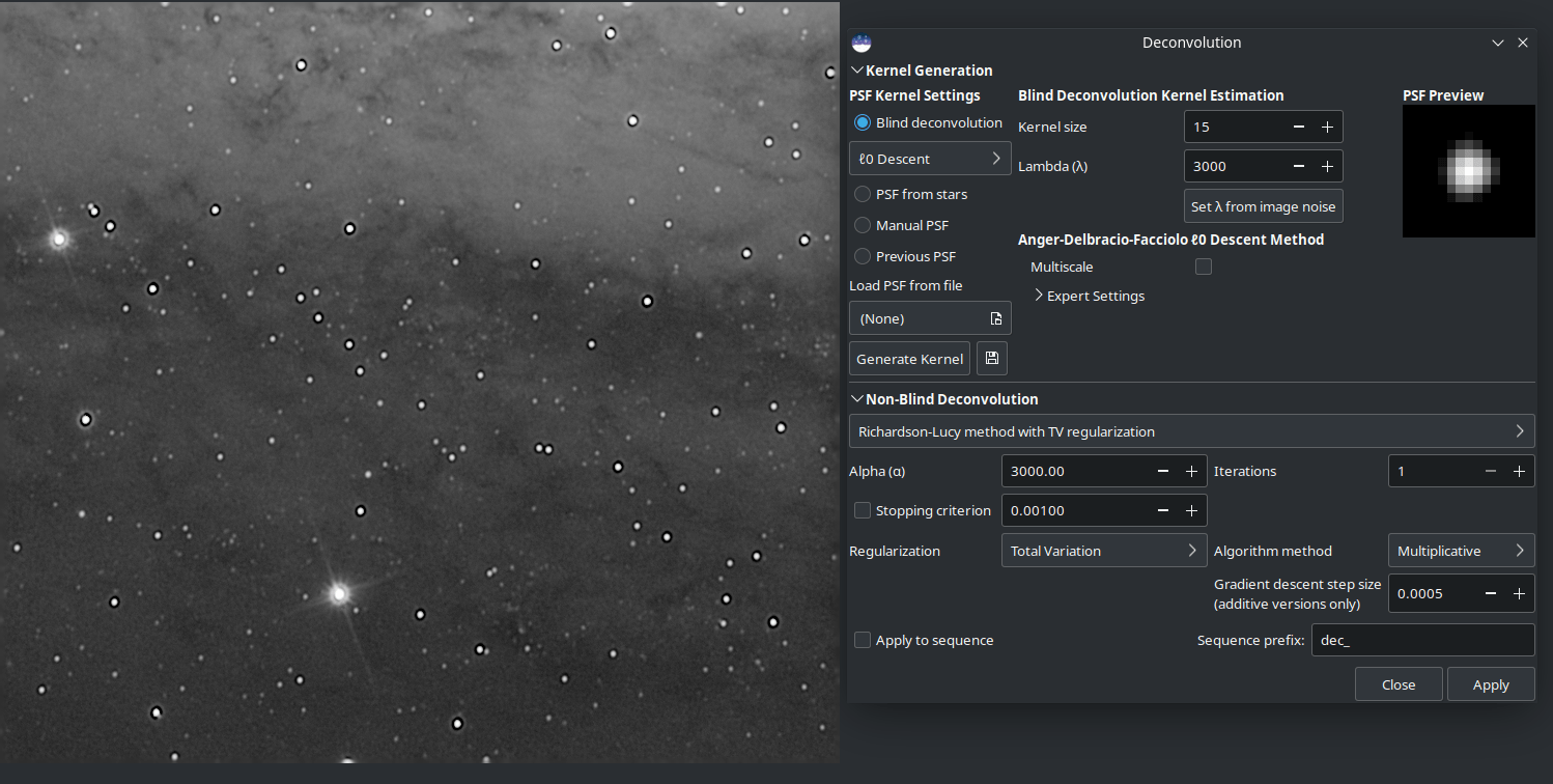
Dialog box of the deconvolution tool.
Overview of Usage
To generate a deconvolution PSF, select the required PSF generation method and press Generate PSF. This can be performed separately from the actual deconvolution so that the user can see the effect of changing the PSF parameters.
Siril only generates monochrome PSFs as this is the most common use case and simplifies the user interface. However, three monochrome PSFs can be saved and composited to produce a 3-channel PSF which can be loaded and used to deconvolve 3-channel images.
To apply deconvolution to a single image, select the required PSF generation method and press Apply. If a blind PSF estimation method has previously been run, the method will automatically be set to Previous PSF, in order to avoid unnecessarily recalculating the PSF.
To apply deconvolution to a sequence, proceed as above but ensure that you activate the Apply to Sequence checkbox. You may also specify a custom prefix to give to the output sequence: if no other prefix is provided, the default (
dec_) will be used.When deconvolving a sequence, the PSF will be calculated only for the first image. The same PSF will be re-used for all images in the sequence.
Overview of Blur Kernel Definition Methods
\(\boldsymbol{ℓ_0}\) Descent: This is the default PSF estimation method based on work by Anger, Delbracio and Facciolo. The parameters do not generally require adjustment, except that for particularly large PSFs you may wish to try the multiscale PSF estimation model. Multiscale is off by default as during development it was noted to have a tendency to produce rather unnatural results with the more common small to medium PSF sizes.
Spectral Irregularities [Goldstein2012]: This PSF estimation method is offered as an alternative. In general it does not perform as well as the \(ℓ_0\) descent method, however it may be useful if you discover an image where the default method does not give good results. For this method the latent sharp image needs not to contain any edges as long as the spectral decay model is respected. On the other hand, the \(ℓ_0\) descent assumes a similar model (since edges have the same spectral decay), but requires to have sparse gradients and be contrasted, thus edges to be in-phase, so theoretically this model may work better on low contrast starless images. Some experimentation is likely required to find the algorithm that best fits your data.
PSF From Stars: This method models a PSF from the average PSF of the selected stars. It is important to be selective about the stars you choose: they must not be saturated as that would give a gross distortion of the PSF estimate, but they must also not be so faint that Siril's star analysis functions provide inaccurate measurements of the stars. The stars chosen should be reasonably bright, fairly central to the image and in an area of the image with a fairly constant background. Once stars are selected, you can pick either a Gaussian or Moffat star profile model and when executing the deconvolution the PSF will be synthesized from the average parameters of the selected stars. If no stars are selected, Siril will attempt to autodetect stars with a peak amplitude between 0.07 and 0.7, with a Moffat profile. This range avoids saturated stars as well as those that are too faint to give an accurate solution, and generally provides good results.
Manual PSF: This method allows you to define a PSF manually. Gaussian, Moffat or disc PSF models can be defined. Note that the FWHM is specified in pixels, not arc seconds. The Gaussian and Moffat models are suitable for deconvolving the shapes of stars resulting from atmospheric distortion; the disc PSF model is suitable for deconvolving the effect of being slightly out of focus.
Load PSF from file: This method allows you to load a PSF from any image format supported by Siril. The provided PSF must be square (it will be rejected if not square) and should be odd (it will be cropped by one pixel in each direction if not odd, but this will give a slightly off-centre PSF and is not optimal compared with providing an odd PSF in the first place). Either monochrome or 3-channel PSFs may be loaded. If a 3-channel PSF is loaded in conjunction with a monochrome image, the evenly-weighted luminance values of the PSF will be used. If a 3-channel PSF is loaded together with a 3-channel image then each channel of the image will be deconvolved using the corresponding channel of the PSF. If a monochrome PSF is loaded together with a 3-channel image then the image will be converted to the LAB colour space and the L (Luminance) channel will be deconvolved using the monochrome PSF for computational efficiency, and the deconvolved L will be recombined with the A and B channels and converted back to RGB.
Previous PSF: This method allows reuse of the previously estimated PSF. It is mostly of use with the blind PSF estimation methods: if you are content with the estimated PSF but wish to make a number of test runs using different parameters for the final stage of deconvolution, you can reuse the previous PSF and save some computation time.
Once estimated, PSFs may be saved if desired. If Siril is compiled with libtiff support then the PSF will be saved in 32-bit TIFF format, with the same filename as the current image but date-and-time-stamped and suffixed with
_PSF. If Siril has been built without libtiff support, the PSF will be saved as a FITS file. While this is Siril's primary format for astronomical image files, TIFF is preferred for PSFs: the disadvantage of using the FITS format for PSFs is potential reduced compatibility with image editors that you may wish to use to edit or examine the saved file.
Tip
If the blind generation of a deconvolution PSF can be done on linear and non-linear data, the use of a PSF from star PSF can only be done on linear images. Otherwise the PSF values would not be valid.
Tip
If a ROI is set, blind PSF estimation methods will calculate the PSF from the ROI rather than the whole image. If you do wish to calculate a PSF from the whole image you must clear the ROI before estimating the PSF, then set the ROI to apply a preview. However, you also have the option of calculating the PSF only from a selected part of the image. This may be desirable if you have optical aberrations close to the edge of the image and wish to estimate the PSF from the central area only.
Overview of Non-Blind Deconvolution
Richardson-Lucy Deconvolution [Lucy1974]: This is the default non-blind deconvolution algorithm. It is an iterative method, famous for its use in correcting image distortions in the early operating period of the Hubble Space Telescope, and in Siril is regularized using either the Total Variation method, which aims to penalize the algorithm for amplifying noise, or the Frobenius norm of the local Hessian matrix. This regularization is based on second derivatives. As well as regularization an early stopping parameter is provided, which allows the algorithm to be halted early once its rate of convergence falls below a certain level. Increasing the value of the early stopping parameter can reduce ringing around stars and sharp edges. Two formulations of the Richardson-Lucy algorithm are provided: the multiplicative formulation and the gradient descent formulation. The latter can allow better control, as the gradient descent step size can be altered (the downside of this is that by using more small steps, more iterations are required to reach the same level of convergence). The bigger advantage of the gradient descent method is that it allows more regularization to be used - this can be problematic in the multiplicative Richardson-Lucy algorithm as the regularization term appears in the denominator and small values here (strong regularization) can cause instability. Siril will use naive convolution for small kernel sizes and FFT-based convolution for larger kernel sizes where FFTs provide a more efficient algorithm. (This is automatic and requires no user intervention.)
Wiener Filtering Method: This method is a non-iterative deconvolution method. It models an assumed Gaussian noise profile, i.e. noise modelled by a constant profile. The constant alpha is used to set the regularization strength in relation to the noise level. As with the other algorithms, a smaller value of alpha provides more regularization. This algorithm can be good for lunar images where the noise regime is Gaussian not Poisson, but usually works badly on deep space imagery where the noise still tends to have a Poisson character.
Split Bregman Method: This method is used internally within the blur PSF estimation processes, and is also offered as a final stage deconvolution algorithm. It is a commonly used algorithm in solving convex optimization problems. This algorithm is also regularized using a total variation cost function. It does not perform as well as Richardson-Lucy on starscapes but may be considered for starless images or lunar surface images.
Tip
Choice of deconvolution method is very important to obtaining good results. Generally for DSO images it is important to use a Richardson-Lucy method: both the Split Bregman and Wiener methods give poor results around stars because of the extreme dynamic range. For linear images it is usually best to use the gradient descent Richardson-Lucy methods, and if ringing occurs around bright stars then reduce the step size. This approach reduces the impact of each iteration therefore more iterations are required, but it does mean that you can achieve finer control taking deconvolution just up to the point where artefacts start to form and then backing off very slightly. For stretched images the multiplicative Richardson-Lucy algorithms may be used.
Tip
For stacked lunar and planetary images the Split Bregman or Wiener methods can be more appropriate. These methods do not generally require iteration in the way that Richardson-Lucy does, and they may be better suited to the noise characteristics of stacked, high signal-to-noise ration images. (The Richardson-Lucy algorithm is based on an assumption of Poisson noise, which is usually true for DSO imaging, whereas the Wiener method implemented here assumes a Gaussian noise distribution which may fit stacked planetary / lunar images better).
Parameters and Settings
General Settings
PSF size. The input PSF size should be chosen sufficiently large to assure that the PSF is included in the specified domain. However, setting it too large can result in a poorer and more time-consuming result from the blind PSF estimation methods.
Lambda (\(\lambda\)). Regularization parameter for PSF estimation. Try decreasing this value for noisy images.
\(\boldsymbol{ℓ_0}\) descent PSF estimation settings
Multiscale. This setting enables multiscale PSF estimation. This may help to stabilize the PSF estimaate when specifying a large PSF size, but some PSFs generated with this option can give rise to unnatural looking results and it is therefore off by default.
Expert settings. These should not normally require adjustment, but are made available for the curious.
Gamma sets the regularization strength used when carrying out the sharp image prediction step. For a given gamma, as the noise increases the estimation also gets noisier. If gamma is increased, the estimation is less affected by noise but tends to be smoother. The default value of 20 was determined experimentally in [Anger2019].
Iterations sets the number of iterations used in the PSF estimate procedure. The authors of the algorithm report that there is minimal benefit in increasing this to 3 and no benefit at all in increasing it beyond 3.
Lambda ratio and lambda minimum sets the parameters for refining the sharp image prediction through successive values of the sharp image predictor regularization parameter at each iteration of the method.
Scale factor, upscale blur and downscale blur are only used when multiscale estimation is active. These set the default scale factor between each scale level and the amount of blurring to use when rescaling between each scale.
Kernel threshold. Values below this level in the PSF estimate are set to zero.
Spectral Irregularity PSF estimation settings
Compensation factor controls the strength of a filter used to avoid excessive sharpness in the estimated PSF. For images with intrinsic blur, a value close to unity should be used. For intrinsically sharp images, low values can result in artefacts and the value should be increased to a large number, effectively disabling the filter.
Expert settings. These should not normally require adjustment, but are made available for the curious.
Inner loop iterations sets the number of iterations performed in the inner loop of the spectral irregularity method. The algorithm converges quickly and it may be possible to reduce this to approximately 100 without much degradation of the result.
Samples per outer loop. This controls how many random phases should be sampled. Because the phase retrieval starts with random values for each sample, it is important to draw enough samples to avoid converging to a local minimum. The PSF stabilizes quickly for low noise images, but if looking for improved results from this method, this is the first of the expert settings to try adjusting especially with images with higher noise levels.
Outer loop iterations. [Anger2018], suggests that 2 iterations can be enough to produce a plausible PSF estimate, and there is negligible value in increasing this above 3.
PSF from Stars
This PSF generation method has no adjustable parameters. It generates a PSF based on the average parameters of the selected stars, using the findstar command or the Dynamic PSF dialog. The average parameters are shown in the deconvolution dialog when this PSF generation method is selected. It is preferable for the user to actively select the stars they wish to use for this method, to obtain the most accurate PSF. Ideally around 10 fairly bright but not saturated stars should be selected from the central region of the image (to exclude stars that may suffer from coma or other aberrations). However, if the user has not selected any stars, Siril will attempt to autodetect suitable stars by running its detection routine with filters set to keep only stars with peak amplitudes between 0.07 and 0.7. This range avoids both saturated stars and those that are too faint to give an accurate solution. It will work well in most cases but may still be affected by off-centre aberrations.
If you select the Symmetrical PSF checkbox, the generated PSF will be circular. This will match the average FWHM and beta of the selected stars but will not match any elongation.
Manual PSF
This PSF generation method allows specification of a custom parametric PSF.
Profile type allows choice of PSF profile. Gaussian, Moffat, disc and Airy disc PSFs are supported.
Gaussian and Moffat PSFs are used for matching star parameters measured from the image. They should provide a good estimate of the total blur function being applied to the image, as stars are point sources.
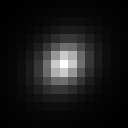
An example of Moffat PSF with fwhm=5", Angle=45°, Ratio=1.20, \(\beta=4.5\) and a PSF size of 15.
Disk PSFs are used to deconvolve images that are out of focus.
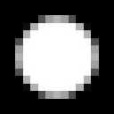
An example of Disk profile with fwhm=5" and a PSF size of 15.
Airy disc PSFs are used to deconvolve the diffraction that arises as a physical consequence of diffraction by the aperture of your telescope.
An example of an Airy-Disk PSF with Diameter=250mm, Focal Length=4500mm, Wavelength=525nm, Pixel Size=2.9µm, Central Obstruction=40% and a PSF size of 41.
FWHM specifies the full width at half maximum of the chosen profile (for disc PSFs it simply specifies the radius).
Beta (\(\beta\)) specifies the beta parameter used in the Moffat PSF profile. It is ignored for other PSF profiles.
For Airy disc PSFs a number of parameters of your telescope and sensor are required:
Aperture
Focal length
Sensor pixel size
Central wavelength being imaged. Siril will try to extract this data from your image metadata where available, but if some parameters are missing or look unreasonable Siril will highlight them and print a warning in the log recommending you check them. The ratio of the central obstruction is also required to generate an accurate Airy disc. This is expressed as a percentage, i.e. the total area of the central obstruction divided by the total area of the aperture x 100. For refractors this is zero; for other telescopes it varies: it may be around 20% for a Newtonian reflector or as much as 40-50% for some Corrected Dall-Kirkham telescopes. You will need to measure your instrument or consult the manufacturer's specifications.
Richardson-Lucy Deconvolution
The parameters used to configure Richardson-Lucy deconvolution in Siril are as follows:
alpha sets the regularization strength. A smaller value of alpha gives stronger regularization and a smoother result; a larger value reduces the regularization strength and preserves more image detail, but may result in the amplification of noise.
Iterations specifies the maximum number of iterations to use. In the absence of noise, a large number of iterations will cause deconvolution to converge the estimate closer to the true image, however an excessively large number of iterations will also magnify noise and cause ringing artefacts around stars. The default is 1 iteration: a higher number can be set to compute multiple iterations automatically, or you can keep pressing Apply to apply one iteration at a time until you are happy with the result. (Or go one further, decide you're no longer happy and use Undo.)
Stopping criterion sets a convergence criterion based on successive estimate differences. This will stop the algorithm once convergence is within the specified limit. This is an important parameter - if you are getting rings around stars in your fnal image, try increasing the value of the stopping criterion. This may be disabled altogether using the check button.
Algorithm method specifies whether to use the multiplicative implementation or the gradient descent implementation.
Step size specifies the step size to use for the gradient descent implementation. Do not set it too large or the algorithm will not converge. This parameter has no effect if the multiplicative implementation is selected.
Tip
For linear images, try using the gradient descent methods provide the control necessary to prevent ringing around stars. For deconvolving stretched images, however, this can be unnecessarily slow, so using the multiplicative methods can often save time without compromising image quality.
Split Bregman Deconvolution
The parameters used to configure Split Bregman deconvolution in Siril are as follows:
alpha sets the regularization strength. A smaller value of alpha gives stronger regularization and a smoother result; a larger value reduces the regularization strength and preserves more image detail, but may result in the amplification of noise.
Iterations specifies the maximum number of iterations to use. The Split Bregman method does not require multiple iterations in the form implemented here, but may be iterated if desired. This generally makes only a small difference and therefore defaults to 1.
Wiener Deconvolution
Wiener deconvolution in Siril only requires one parameter:
alpha sets the regularization strength. A smaller value of alpha gives stronger regularization and a smoother result; a larger value reduces the regularization strength and preserves more image detail, but may result in the amplification of noise.
FFTW Performance Settings
The PSF estimation and deconvolution algorithms make extensive use of fast Fourier transforms using the FFTW library. This offers a number of tuning options, which can be adjusted in the performance tab of the main Siril preferences dialog.
Note on Image Row Order
Different types of image processed by Siril can have their pixel data arranged in different orders. SER video files always store data top down, whereas FITS files may store data either bottom up or top down. Bottom up is the original recommendation, however increasingly FITS are sourced from CMOS cameras which tend to follow a top down pixel order.
When an image is deconvolved with a PSF created from the same image (or with it open) this causes no problem. However there is potential for problems to arise if a PSF is generated with an image with one row order and used to deconvolve an image or sequence with the opposite row order. This is a niche use case, but handling it consistently results in behaviour which at first sight can be surprising: it is therefore explained below.
Siril handles the issue by tracking the row order of the image the PSF was created with. PSFs are always saved using a bottom up row order (automatically flipping them if they were created with a top down image), and when loaded the row order is matched to the row order of the currently open image. If an image of the opposite row order is opened, the row order of the PSF will be changed to match. This means that if, for example, you take some bottom up FITS images, use one of them to generate a PSF, and then convert them to a top down SER sequence, the PSF will be converted to the correct orientation to match the SER sequence. If a PSF is being previewed at the time an image with the opposite row order is opened the preview will not update immediately: the row order change will be detected automatically and the PSF flipped at the time when it is applied to the image.
Rogues' Gallery
This section shows some examples of where deconvolution has gone wrong, together with explanations of why.

The manually specified PSF was too big, resulting in large dark rings around stars.
Too many iterations have been applied. (I applied them one at a time to exaggerate the result, which is why the iterations parameter still says 1.)
Close-up showing the effect of trying to apply too much regularization (alpha = 30) using the multiplicative version of Richardson-Lucy. For strong regularization and / or better control over each iteration, the gradient descent formulation is recommended.
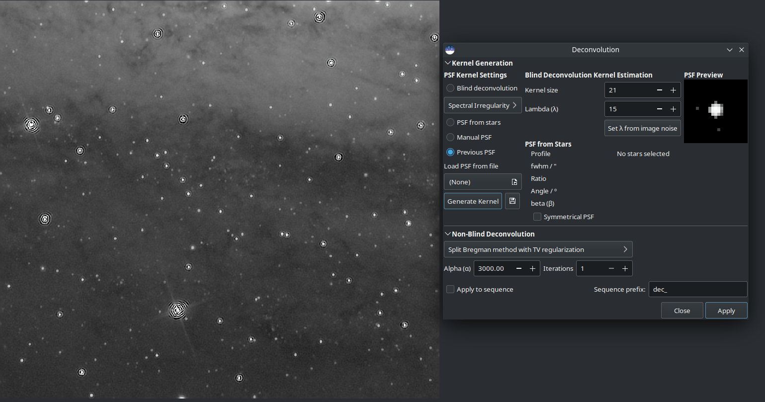
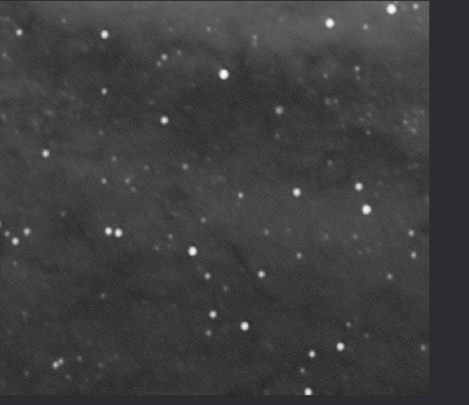
Typical example of attempting to deconvolve an unstretched starfield using Split Bregman (in this case) or Wiener filter deconvolution. Those are better for planetary / lunar / solar images; for starscapes Richardson-Lucy is always recommended.
Deconvolution: Usage Tips
You've arrived here from the hints button in the deconvolution tool in Siril. No worries: deconvolution is a tricky technique. Even theoretically, it's really hard: there are no guarantees the maths will always converge to a unique solution that improves your image. That said, here are some tips to help you get the most out of Siril's deconvolution algorithms.
What PSF to use?
Using an accurate PSF is fundamental to achieving good results from deconvolution. The two simplest ways to generate a PSF are to use a blind PSF estimate, or to model your PSF on stars in your image.
PSF from Stars
Siril can detect and model stars in your image. See the Dynamic PSF help page for details. To get a good model for your PSF, try selecting the Moffat star profile in Dynamic PSF. Stars are point sources so the spread function of an average star is a good model for the blurring effects that we are trying to remove by deconvolution.
Tip
Once you have detected stars, sort them by peak amplitude (parameter "A"). Select and delete any with amplitude greater than 0.7 or less than 0.1, and if your image contains background galaxies check that no false positives remain. Stars in this brightness range are not saturated and not too faint to give an accurate PSF model.
Tip
If the blind generation of a deconvolution PSF can be done on linear and non-linear data, the use of a PSF from star PSF can only be done on linear images. Otherwise the PSF values would not be valid.
Blind PSF Estimate
These methods can automatically estimate a PSF based on the image itself. If you have no better prior knowledge of the PSF such as stars in the image (for example, lunar imagery that contains no stars) then this may be your best option. In most cases it is recommended to use the default \(\boldsymbol{ℓ_0}\) method: it is faster and usually gives better results.
Tip
However you are generating your PSF, check the preview to make sure that it does not look cropped. If it does, increase the PSF size until no significant parts of the PSF are cropped.
Other PSF Generation Methods
Other PSF generation methods worthy of mention are the manual disc profile and the Airy disc. The disc profile can be used to improve images where the focus is slightly off. Try to match the size of the disc to the size of the out-of-focus blur. The Airy disc can be used to fix the slight blurring caused by the diffraction of the telescope tube itself.
Tip
If you have exceptional seeing (little to no atmospheric blur) deconvolving the image using an Airy disc may be all that you need.
Deconvolving the Image
Once you've generated a PSF you're happy with, you're ready to deconvolve your image. It is important to use the right settings to get good results.
Tip
Deconvolution is quite slow for large images. To make it quicker to find the best parameters, save your work at this point and use the ROI feature.
Images with Stars
Images containing stars, especially linear (unstretched) data, should always be deconvolved using the Richardson-Lucy methods. Ignore Split Bregman and Wiener: those algorithms are suited to solar system images.
Deep space images pose 2 challenges with deconvolution: ringing around bright stars, and noise amplification in the background.
To deal with rings around stars, try using the Gradient Descent method and increase the number of iterations gradually until you start to see signs of dark rings forming around stars, then reduce the iterations just a little.
The above animation shows the effect of reducing the numebr of iterations of the multiplicative formulation of Richardson-Lucy: it also demonstrates the finer control that can be achieved by using the gradient descent method, at the cost of more iterations.
To deal with amplification of background noise, you can try applying a little noise reduction before deconvolution. In the Noise Reduction dialog, choose the Anscombe VST secondary denoising algorithm and leave the modulation quite low, try around 50-60%. You just want to take the edge off the noise to allow you to push the number of iterations a little further, not generate a completely smooth image.
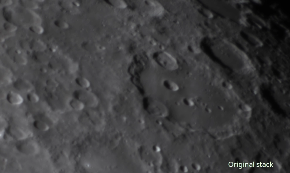
Lunar Images
Typically you may wish to sharpen a lunar image after stacking. Stacked lunar images can be sharpened very nicely using the Split Bregman or Wiener methods. My usual choice is Split Bregman. Try leaving the value of \(\boldsymbol{\alpha}\) at the default, and deconvolving the image using a blind estimated \(\boldsymbol{ℓ_0}\) PSF. An example of this is shown below using a freshly stacked lunar image (i.e. no wavelet processing has been done to it). Despite the limitations of the GIF animation format the sharpening can clearly be seen; it is also clear that the results from Split Bregman and Wiener are very similar.
Stacked Planetary Images
A typical planetary workflow involves stacking the planetary SER video in a specialist tool such as Autostakkert! or Astrosurface, and then sharpening the resulting image using wavelets and deconvolution. A combination of Siril's A trous Wavelets tool and the Deconvolution tool gives excellent results as shown here. This image of Jupiter was initially sharpened using wavelets with the first layer control set to 75, the second set to 10 and the others all left at the default. A colour PSF was then built from 3 Airy discs calculated for the telescope and sensor used (a 6" Newtonian with a 3x Barlow lens and an ASI462MC sensor with 2.9 micron pixels) composited using the RGB composition tool. This was used to deconvolve the image with 6 iterations of Richardson-Lucy (here I used the multiplicative version). At each step the image becomes sharper.

Raw stack, still blurry.

Processed with Siril wavelet decomposition, wavelet layer 1 strength 75, wavelet layer 2 strength 10.

Processed with Siril wavelets as above, and then with 6 iterations of multiplicative Richardson-Lucy deconvolution.
Unstacked Planetary Sequences
Tip
Warning: this method is extremely slow as it requires individual processing of typically 30,000 (or more) images in a planetary sequence!
Some users have suggested mitigating telescope diffraction pre-stacking by deconvolving your sequence using an Airy disc PSF. To do this with a typical one-shot colour planetary camera, the sequence has to be set to debayer on load. You can take this one step further if you wish by generating three separate Airy discs for red, green and blue wavelengths (typically 600nnm, 530nm and 450nm respectively). Siril cannot directly generate a colour PSF (the deconvolution UI is busy enough!) but if you save each of the red, green and blue Airy discs separately you can combine them into a colour PSF using the RGB composition tool. Save this, and if a colour or sequence is loaded the PSF will load in colour and will deconvolve each colour channel using the appropriate PSF.
Stacked and sharpened without individually deconvolving frames.
Raw stack: best 30% of 91k frames individually deconvolved using Siril.
Result of sharpening the individually deconvolved stack.
In the image above a slight improvement to the shape of the edge is evident in the version that was frame-by-frame deconvolved with an Airy disc PSF using Siril's Richardson-Lucy method prior to stacking, but care must be taken to avoid loss of details. This process is very slow: my development machine took 4.5 hours to deconvolve each of the 91k frames in this sequence, and the improvement may be minor if any.
Commands
Siril command line
makepsf clear
makepsf load filename
makepsf save [filename]
makepsf blind [-l0] [-si] [-multiscale] [-lambda=] [-comp=] [-ks=] [-savepsf=]
makepsf stars [-sym] [-ks=] [-savepsf=]
makepsf manual { -gaussian | -moffat | -disc | -airy } [-fwhm=] [-angle=] [-ratio=] [-beta=] [-dia=] [-fl=] [-wl=] [-pixelsize=] [-obstruct=] [-ks=] [-savepsf=]
Siril command line
rl [-loadpsf=] [-alpha=] [-iters=] [-stop=] [-gdstep=] [-tv] [-fh] [-mul]
Siril command line
sb [-loadpsf=] [-alpha=] [-iters=]
References
Anger, J., Facciolo, G., & Delbracio, M. (2018). Estimating an image's blur kernel using natural image statistics, and deblurring it: an analysis of the Goldstein-Fattal method. Image Processing On Line, 8, 282-304. https://doi.org/10.5201/ipol.2018.211
Anger, J., Facciolo, G., & Delbracio, M. (2019). Blind image deblurring using the l0 gradient prior. Image processing on line, 9, 124-142. https://doi.org/10.5201/ipol.2019.243
Goldstein, A., & Fattal, R. (2012, October). Blur-kernel estimation from spectral irregularities. In European Conference on Computer Vision (pp. 622-635). Springer, Berlin, Heidelberg. https://doi.org/10.1007/978-3-642-33715-4_45
Lucy, L. B. (1974). An iterative technique for the rectification of observed distributions. The astronomical journal, 79, 745. https://doi.org/10.1086/111605.