Hintergrund-Extraktion

The sky background often has an unwanted gradient caused by light pollution, the moon, or simply the orientation of the camera relative to the ground. This tool models that gradient and removes it, following a smooth function so that nebulae and other real signal are preserved.

Siril offers two methods to build the background model, selected with the Method drop-down at the top of the dialog:

• Sample-based (the classic method): the background is sampled at many places of the image, either on a regular grid or at manually placed points, and a smooth surface is interpolated through those samples.

• Automatic (sample-free): no samples are placed. The background is fitted directly on every pixel that survives an iterative robust rejection of structures (stars, nebulae), which makes it convenient when placing a good sample grid is difficult.

The Correction mode, the Compute Background button and the View selector (see General settings) are common to both methods. All the other options are specific to the method selected.

Sample-based method

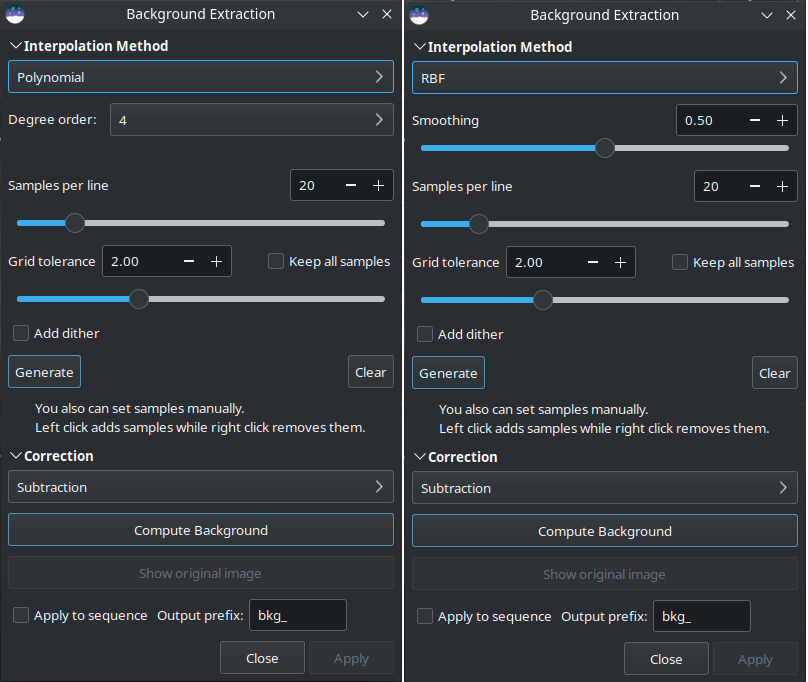
Dialogbox Hintergrund-Extraktion. Auf der linken Seite ist die Polynom-Version zu sehen, rechts RBF.

Proben können automatisch platziert werden, indem Sie eine Dichte angeben (Proben pro Zeile) und auf Generieren klicken. Wenn Bereiche des Bildes um einen Faktor Rastertoleranz mal Sigma heller als der Median sind, wird dort keine Probe platziert.

There are some options regarding how to place samples.

• The default is a regular grid, however you can select random sample locations to achieve the same sample positioning as SetiAstro's AutoDBE process.

• You can select sample optimization. If this is enabled, the position of each sample will be optimized by seeking a local minimum sample median. This may result in an irregular grid. Note that this setting also affects manually placed samples, so don't be surprised if your samples move! If you wish to place a sample precisely then disable this.

You can also limit the area in which samples are placed. If a sample lands too close to the image edge it may include black border areas, or areas of uneven coverage, resulting in a poor background model. By making a selection a little in from the image edge, you can restrict the sample placement to inside the selection thus eliminating the problem with edge samples.

Tipp

Wenn Sie sehr starke Gradienten haben, zum Beispiel bei Aufnahmen unter einem Stadthimmel mit hohem Bortle-Wert, reicht möglicherweise selbst die maximale Gittertoleranz nicht aus. In diesem Fall können Sie das Kontrollkästchen „Alle Proben behalten“ aktivieren und das gesamte Probenraster wird ausgefüllt. Anschließend müssen Sie manuell Proben von tatsächlichen astronomischen Objekten entfernen.

After generation, samples can also be added manually (left click) or removed manually (right click).

• Add dither: check this option when color banding is produced after background extraction. Dither is an intentionally applied form of noise used to randomize quantization error, preventing large-scale patterns such as color banding in images.

There are two algorithms to interpolate the background model through the samples:

RBF

Dies ist die modernste Methode. Es verwendet die Radiale Basisfunktion <https://de.wikipedia.org/wiki/Radiale_Basisfunktion>, um einen Himmelshintergrund zu synthetisieren und den Farbverlauf mit großer Flexibilität zu entfernen. Es erfordert einen einzelnen Parameter, der in Form eines Schiebereglers vorliegt: Glätten. Mit diesem Wert können Sie bestimmen, wie weich oder hart der Übergang zwischen den Abtastpunkten berechnet wird. Bei großen und gleichmäßigen Verläufen ist ein hoher Glättungsfaktor sinnvoll, bei kleinen, lokalen Verläufen ein entsprechend niedrigerer Wert.

Tipp

Beginnen Sie mit der Grundeinstellung (50 %) und optimieren Sie diese schrittweise, um optimale Ergebnisse zu erzielen.

Theorie

Radiale Basisfunktionen sind Funktionen der Form \(\phi(\mathbf{x}) = \phi(\| \mathbf{x} \|)\), wobei wir in unserem Fall die euklidische Norm \(\| \mathbf{x} \| = \sqrt{x_1^2 + x_2^2}\) verwenden. Die Funktion \(f\), die das Hintergrundmodell beschreibt, kann nun als lineare Kombination ausgedrückt werden

\[f(\mathbf{x}) = \sum_i w_i \, \phi(\|\mathbf{x} - \mathbf{x_i}\|) + o\]

wobei \(w_i\) den Gewichtungen für die verschiedenen Stichprobenpunkte entspricht und \(o\) einem konstanten Offset entspricht.

Die Anforderung, dass die Funktion \(f\) die Beispielpunkte durchlaufen soll, führt zu der Bedingung

\[\begin{split}\begin{pmatrix} \phi(\mathbf{x}_1 - \mathbf{x}_1) & \phi(\mathbf{x}_1 - \mathbf{x}_2) & \dots & \phi(\mathbf{x}_1 - \mathbf{x}_N) & 1 \\ \phi(\mathbf{x}_2 - \mathbf{x}_1) & \phi(\mathbf{x}_2 - \mathbf{x}_2) & \dots & \phi(\mathbf{x}_2 - \mathbf{x}_N) & 1 \\ \vdots & \vdots & \ddots & \vdots \\ \phi(\mathbf{x}_N - \mathbf{x}_1) & \phi(\mathbf{x}_N - \mathbf{x}_2) & \dots & \phi(\mathbf{x}_N - \mathbf{x}_N) & 1 \\ 1 & 1 & \dots & 1 & 0 \end{pmatrix} \begin{pmatrix} w_1 \\ w_2 \\ \vdots \\ w_N \\ o \end{pmatrix} = \begin{pmatrix} y_1 \\ y_2 \\ \vdots \\ y_N \\ 0 \end{pmatrix} \, ,\end{split}\]

was nur erfüllt werden kann, wenn die Matrix auf der linken Seite invertierbar ist. Mit der richtigen Wahl der Funktion \(\phi\) kann dies immer gewährleistet werden [Wright2003].

Zusätzlich wird der Summand \(s \, I\) zur Matrix auf der linken Seite hinzugefügt, wobei \(s\) ein Glättungsparameter und \(I\) die Einheitsmatrix ist. Der Summand bewirkt eine Regularisierung, die zu einem glatteren Ergebnis führt, je größer der Parameter \(s\) ist. Dieser Parameter kann mit dem Parameter Glätten des Dialogfelds geändert werden.

Für die radiale Basisfunktion verwenden wir den Dünnplatten-Spline \(\phi(|\mathbf{x}|) = |\mathbf{x}|^2 \log(|\mathbf{x}|)\).

Polynomisch

Dies ist der ursprüngliche und einfachste Algorithmus, der in Siril entwickelt wurde. Bei der Polynomberechnung wird nur ein Parameter verwendet: die Ordnung. Je höher der Ordnungsgrad, desto flexibler ist die Korrektur, aber ein zu hoher Grad kann zu seltsamen Ergebnissen wie einer Überkorrektur führen.

Tipp

Eine Korrektur der Stufe 1 kann sehr nützlich sein, wenn Sie den Farbverlauf auf den Subs/Lights entfernen möchten.

Warnung

Hintergrundentfernen kann auch an CFA-Bildern durchgeführt werden, aber nur an solchen, die ein Bayer-Muster haben. (Es ist nicht für X-TRANS Muster unterstützt) Bilder mit Bayer-Muster, werden als vier getrennte Bilder behandelt, jedes korrespondiert mit einem CFA-Unterkanal. Jeder Unterkanal wird unabhängig voneinander verarbeitet. Dann werden sie wieder in das originale Muster zusammengeführt.

Die vorgesehene Nutzung dafür ist das Entfernen von linearen Gradienten von Sequenz-Frames vor dem Anwenden von Drizzle auf eine Sequenz mit Bayer-Muster. In diesem Fall wird empfohlen, eine lineare (ploynomialer Grad 1) Gradient-Entfernung wie mit anderer Gradient-Entfernung, die vor dem Stacken angewendet wird.

Theorie

Polynomfunktionen sind Funktionen der Form

\[\begin{equation} f(x)=a_nx^n+a_{n-1}x^{n-1}+\cdots+a_2x^2+a_1x+a_0 \end{equation}.\]

In Siril ist der maximal zulässige Grad \(n=4\) und kann über das Dropdown-Menü Ordnung geändert werden. Darüber hinaus ist das Modell im Allgemeinen instabil und liefert schlechte Ergebnisse.

Automatic (sample-free) method

When Automatic (sample-free) is selected in the Method drop-down, no samples are placed on the image. Instead, the background is fitted directly on the pixels: the tool iteratively rejects everything that does not look like background (stars, nebulae and other structures) and fits a smooth model on the pixels that remain. This is convenient when a good sample grid is hard to place, for example on densely populated fields.

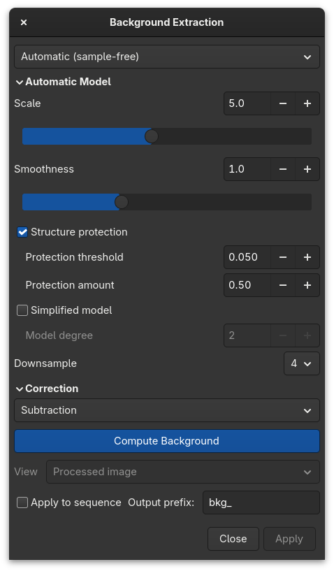
Background extraction dialog with the automatic (sample-free) method selected, showing the Automatic Model panel.

Warnung

The automatic method fits the background over the whole image, borders included. Stacked images very often have black or uneven edges (caused by dithering, field rotation or incomplete overlap between frames). These borders must be cropped away before running the automatic method, otherwise they are treated as extremely dark background and corrupt the model. Unlike the sample-based method, the edges cannot be excluded here by making a selection, so a clean crop of the stacked result is imperative.

The following parameters are available in the Automatic Model panel:

• Scale: relative scale of the multiscale model, in the [1, 10] range (default 5). A higher value keeps only large-scale gradients and gives a smoother model, while a lower value lets the model follow more complex or more local gradients.

• Smoothness: extra smoothing applied to the final model (default 1). A higher value gives a softer, more gradual background; a value of 0 leaves the fitted model untouched.

• Structure protection: when enabled (the default), extended bright structures such as nebulae are masked so that they are not absorbed into the background model. Two sub-parameters control it:

  • Protection threshold: brightness above the model at which a pixel starts to be treated as a structure (default 0.05). A lower value protects more of the image.

  • Protection amount: how far the protection mask grows around the detected structures (default 0.5).

• Simplified model: replaces the multiscale model with a stiff low-degree polynomial. Use it when a nebula fills most of the frame and the default model would hollow it out. Its degree is set with:

  • Model degree: polynomial degree of the simplified model, in the [1, 6] range (default 2). A lower value is stiffer (degree 1 is a plane).

• Downsample: internal working scale factor (1, 2, 4 or 8, default 4). A higher value makes the computation faster but coarser; it does not change the scale of the background itself.

Tipp

Start with the default settings. If real signal (a large nebula) is being eaten by the model, either lower the Protection threshold or switch to the Simplified model with a low Model degree.

Theorie

The automatic model is estimated independently on each channel and, for speed, on an internally downsampled copy of the image (the Downsample factor). It then alternates a fit step and a robust rejection step:

1. An initial background model \(B\) is fitted on every pixel.

2. The residual \(r = I - B\) between the image \(I\) and the current model is computed, and its robust location and scale are estimated from the pixels currently kept, using the median and the median absolute deviation (\(\sigma = 1.4826 \times \mathrm{MAD}\)).

3. Pixels are rejected by an asymmetric sigma clipping: a pixel is kept only if its residual lies within \([\,\mathrm{med} - k_\mathrm{lo}\,\sigma,\ \mathrm{med} + k_\mathrm{hi}\,\sigma\,]\), with a tighter upper bound than the lower one. Bright outliers (stars, nebula cores) are therefore discarded more aggressively than faint ones.

4. When Structure protection is enabled, a spatially-coherent mask of extended bright structures is additionally removed from the fitting set, so large nebulae are not mistaken for background.

5. The model is re-fitted on the surviving pixels and the process repeats until the kept set stabilises.

Two models are available. The default multiscale model rebuilds a smooth surface across the rejected regions by harmonic-style inpainting (repeated low-pass filtering that restores the kept pixels at each pass); the Scale parameter sets the width of that low-pass, i.e. the spatial scale below which variations are considered signal rather than background. The simplified model instead fits a single 2D polynomial of the chosen Model degree by least squares. In both cases a final, optional Gaussian smoothing is controlled by Smoothness.

The low-pass filtering relies on a fast separable Gaussian approximated by variance-matched box blurs, so its cost is independent of the smoothing radius.

Allgemeine Einstellungen

These controls sit below the method panels and apply whichever method is selected.

• Korrektur:

  • Subtraktion: Sie wird hauptsächlich zur Korrektur von additiven Effekten verwendet, z. B. von Gradienten, die durch Lichtverschmutzung oder den Mond verursacht werden.

  • Division: Sie wird hauptsächlich zur Korrektur multiplikativer Phänomene verwendet, wie z. B. Vignettierung oder differentielle atmosphärische Absorption. Diese Art von Operation sollte jedoch besser mit einer Master-Flat-Korrektur durchgeführt werden.

• Compute Background: This will compute the synthetic background and will apply the selected correction. The model is always computed from the original image kept in memory allowing the user to work iteratively. The result is only previewed at this stage; it is committed when you close the dialog with the Apply button.

• View: once a background has been computed, this drop-down chooses what is shown in the main view without recomputing anything:

  • Processed image: the corrected result (the default).

  • Background model: the background that was removed, reconstructed from the original and the processed image.

  • Original image: the untouched image kept in memory.

  This replaces the former Show original image button and works identically for both methods.

Der Hintergrundgradient eines vorverarbeiteten Bildes kann komplex sein, da sich der Gradient mit der Aufnahmesitzung gedreht haben kann. Es kann schwierig sein, ihn vollständig zu entfernen, da es schwierig ist, ihn mit einer Polynomfunktion darzustellen. Wenn dies der Fall ist, können Sie in Erwägung ziehen, den Gradienten in den Einzelframes zu entfernen: In einem Einzelbild ist der Hintergrundgradient viel einfacher und folgt im Allgemeinen einer einfachen linearen Funktion (Grad 1).

Tipp

Manchmal treten nach der Hintergrundextraktion unschöne Farbstreifen auf. In diesem Fall müssen zwei Dinge überprüft werden. Erstens: Wenn es sich um ein 16-Bit-Bild handelt, empfehlen wir Ihnen dringend, immer das 32-Bit-Format zu verwenden. Wenn Sie trotz allem immer noch solche Artefakte beobachten, ist die oben erläuterte Option Dithering hinzufügen die Lösung für Ihr Problem.

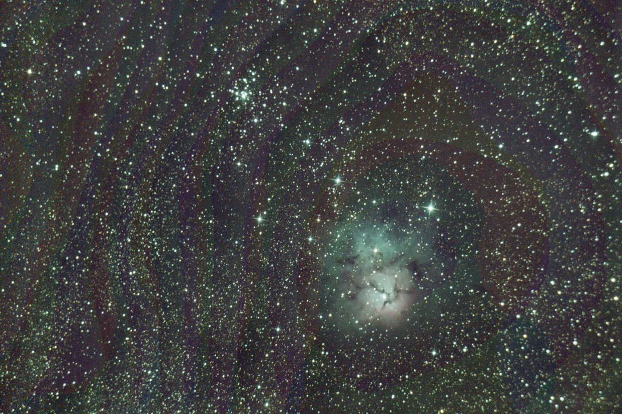
Wenn eine solche Streifenbildung nach der Gradientenextraktion auftritt, kann dies mit der Option Dithering hinzufügen behoben werden (mit freundlicher Genehmigung von Nathan B.).

Tipp

Gute Ergebnisse mit dem RBF-Algorithmus erfordern im Allgemeinen weniger Stichproben als mit dem Polynomalgorithmus.

Siehe auch

Weitere Erklärungen finden Sie in der entsprechenden Anleitung hier (englisch).

Siril Kommandozeile

subsky { -rbf | degree | -auto } [-dither] [-samples=20] [-tolerance=1.0] [-smooth=0.5] [-existing] [-random] [-gradient] [-border=<pixels|percent%>] [-scale=5] [-smoothness=1] [-noprotect] [-protect_threshold=0.05] [-protect_amount=0.5] [-simplified] [-degree=2] [-downsample=4] [-mode=subtract|divide]

Berechnet einen synthetischen Hintergrundgradienten unter Verwendung des Polynomfunktionsmodells des Grades degree oder des RBF-Modells (wenn stattdessen -rbf angegeben wird) und subtrahiert ihn vom Bild.

Die Anzahl der Stichproben pro horizontaler Linie und die Toleranz zum Ausschluss hellerer Bereiche können mit den optionalen Argumenten angepasst werden. Die Toleranz wird in MAD-Einheiten angegeben: Median + Toleranz * mad.

Dithering, das für geringe dynamische Gradienten erforderlich ist, kann mit -dither aktiviert werden.

For RBF, the additional smoothing parameter is also available. To use pre-existing background samples (e.g. if you have set background samples using a Python script) the -existing argument must be used.

-random: place sample points randomly in darker areas of each image quadrant plus fixed border/corner points, instead of using a regular grid. In this mode the -samples value is the total number of interior random points.

-gradient: after placing each sample (grid or random), move it to the nearest local brightness minimum using gradient descent, shifting it away from stars and other bright objects. Can be combined with either placement mode.

-border=: exclude a border strip from sample placement. For a pixel value (e.g. -border=50), the same number of pixels is excluded from all four sides. For a percentage value (e.g. -border=10%), the left and right strips are that percentage of the image width, and the top and bottom strips are that percentage of the image height, so the excluded area is proportional to the image dimensions rather than a fixed pixel count.

-auto: use the automatic, sample-free model instead. It places no samples: the background is fitted on every pixel that survives an iterative robust rejection of structures (stars, nebulae). In this mode the sample-related options are ignored and the following apply:

-scale= relative model scale in the [1, 10] range (higher = smoother, default 5).

-smoothness= extra regularisation of the final model (default 1).

-noprotect: disable structure protection (masking of extended bright structures so they are not absorbed into the model).

-protect_threshold= brightness above the model at which a pixel is treated as a structure (default 0.05).

-protect_amount= how far the protection mask grows around detected structures (default 0.5).

-simplified: replace the multiscale model with a stiff polynomial, best when a nebula fills the frame; -degree= sets its degree in the [1, 6] range (default 2).

-downsample= internal working scale factor, one of 1, 2, 4, 8 (default 4).

-mode= subtract (additive gradient, default) or divide (multiplicative, vignetting/flat)

Tipp

The automatic (sample-free) method is available on the command line with the -auto argument. In this mode the sample-related options are ignored and the automatic-model parameters (-scale=, -smoothness=, -noprotect, -protect_threshold=, -protect_amount=, -simplified, -degree=, -downsample=) apply instead, together with -mode=subtract|divide for the correction type. See the subsky reference above for the full list.

Tipp

The -existing command argument forces use of existing background samples. This option is primarily for use in conjunction with the Python module where SirilInterface.set_bgsamples() can be used to set custom background samples based on user-defined algorithms. If it is not provided, subsky will automatically regenerate background samples. Note that the -existing option is not available with the seqsubsky command, because sequence frames are not necessarily registered at the time background subtraction is carried out, so the samples for one frame do not necessarily apply to another.

Siril Kommandozeile

seqsubsky sequencename { -rbf | degree | -auto } [-nodither] [-samples=20] [-tolerance=1.0] [-smooth=0.5] [-prefix=] [-random] [-gradient] [-border=<pixels|percent%>] [-scale=5] [-smoothness=1] [-noprotect] [-protect_threshold=0.05] [-protect_amount=0.5] [-simplified] [-degree=2] [-downsample=4] [-mode=subtract|divide]

Gleicher Befehl wie SUBSKY, aber für die Sequenz sequencename.

Dithering, required for low dynamic gradients, can be disabled with -nodither. Note that the -existing option is not available for sequence background removal, as the frames of a sequence are not necessarily always aligned.

The output sequence name starts with the prefix "bkg_" unless otherwise specified with -prefix= option. Only selected images in the sequence are processed.

-random and -gradient options are available as in SUBSKY.

-border= is available as in SUBSKY

Verweis: subsky

[Wright2003]

Wright, Grady Barrett. Radial basis function interpolation: numerical and analytical developments. University of Colorado at Boulder, 2003.