Background Extraction

The sky background often has an unwanted gradient caused by light pollution, the moon, or simply the orientation of the camera relative to the ground. This tool models that gradient and removes it, following a smooth function so that nebulae and other real signal are preserved.

Siril offers two methods to build the background model, selected with the Method drop-down at the top of the dialog:

• Sample-based (the classic method): the background is sampled at many places of the image, either on a regular grid or at manually placed points, and a smooth surface is interpolated through those samples.

• Automatic (sample-free): no samples are placed. The background is fitted directly on every pixel that survives an iterative robust rejection of structures (stars, nebulae), which makes it convenient when placing a good sample grid is difficult.

The Correction mode, the Compute Background button and the View selector (see General settings) are common to both methods. All the other options are specific to the method selected.

Sample-based method

Background extraction dialog box. On the left is the polynomial version, on the right RBF.

Samples can be automatically placed by providing a density (Samples per line) and clicking on Generate. If areas of the image are brighter than the median by some factor Grid tolerance times sigma, then no sample will be placed there.

There are some options regarding how to place samples.

• The default is a regular grid, however you can select random sample locations to achieve the same sample positioning as SetiAstro's AutoDBE process.

• You can select sample optimization. If this is enabled, the position of each sample will be optimized by seeking a local minimum sample median. This may result in an irregular grid. Note that this setting also affects manually placed samples, so don't be surprised if your samples move! If you wish to place a sample precisely then disable this.

You can also limit the area in which samples are placed. If a sample lands too close to the image edge it may include black border areas, or areas of uneven coverage, resulting in a poor background model. By making a selection a little in from the image edge, you can restrict the sample placement to inside the selection thus eliminating the problem with edge samples.

Truco

If you have very strong gradients, for example when imaging in high Bortle urban skies, even the maximum grid tolerance may be insufficient. In this case you can check the Keep all samples checkbox and the full sample grid will be populated. You will then need to remove samples from actual astronomical objects manually.

After generation, samples can also be added manually (left click) or removed manually (right click).

• Add dither: check this option when color banding is produced after background extraction. Dither is an intentionally applied form of noise used to randomize quantization error, preventing large-scale patterns such as color banding in images.

There are two algorithms to interpolate the background model through the samples:

RBF

This is the most modern method. It uses the radial basis function to synthesize a sky background to remove the gradient with great flexibility. It requires a single parameter which is present in the form of a slider: Smoothing. With this value you can determine how soft or hard the transition between the sample points is calculated. A high smoothing factor makes sense for large and uniform gradients, and a correspondingly lower value for small, local gradations.

Truco

Start with the basic setting (50%) and gradually tweak for optimal results.

Theory

Radial basis functions are functions of the form \(\phi(\mathbf{x}) = \phi(\| \mathbf{x} \|)\), whereby in our case we use the Euclidean norm \(\| \mathbf{x} \| = \sqrt{x_1^2 + x_2^2}\). The function \(f\), which describes the background model, can now be expressed as a linear combination

\[f(\mathbf{x}) = \sum_i w_i \, \phi(\|\mathbf{x} - \mathbf{x_i}\|) + o\]

where \(w_i\) corresponds to the weights for the different sample points and \(o\) corresponds to a constant offset.

The requirement that the function \(f\) should pass through the sample points results in the condition

\[\begin{split}\begin{pmatrix} \phi(\mathbf{x}_1 - \mathbf{x}_1) & \phi(\mathbf{x}_1 - \mathbf{x}_2) & \dots & \phi(\mathbf{x}_1 - \mathbf{x}_N) & 1 \\ \phi(\mathbf{x}_2 - \mathbf{x}_1) & \phi(\mathbf{x}_2 - \mathbf{x}_2) & \dots & \phi(\mathbf{x}_2 - \mathbf{x}_N) & 1 \\ \vdots & \vdots & \ddots & \vdots \\ \phi(\mathbf{x}_N - \mathbf{x}_1) & \phi(\mathbf{x}_N - \mathbf{x}_2) & \dots & \phi(\mathbf{x}_N - \mathbf{x}_N) & 1 \\ 1 & 1 & \dots & 1 & 0 \end{pmatrix} \begin{pmatrix} w_1 \\ w_2 \\ \vdots \\ w_N \\ o \end{pmatrix} = \begin{pmatrix} y_1 \\ y_2 \\ \vdots \\ y_N \\ 0 \end{pmatrix} \, ,\end{split}\]

which can only be fulfilled if the matrix on the left-hand side is invertible. With the right choice of function \(\phi\) this can always be guaranteed [Wright2003].

In addition, the summand \(s \, I\) is added to the matrix on the left-hand side, where \(s\) is a smoothing parameter and \(I\) is the unit matrix. The summand causes a regularization, which results in a smoother result the larger the parameter \(s\) is. This parameter can be changed with the Smoothing parameter of the dialog box.

For the radial basis function, we use the thin-plate spline \(\phi(|\mathbf{x}|) = |\mathbf{x}|^2 \log(|\mathbf{x}|)\).

Polinómico

This is the original and simplest algorithm developed in Siril. Only one parameter is used in polynomial computation: the Degree order. The higher the degree, the more flexible the correction, but a too high degree can give strange results like overcorrection.

Truco

A degree 1 correction can be very useful for when you want to remove the gradient on the subs.

Advertencia

Background removal can be carried out on CFA images, but only if they have Bayer patterns. (It is not supported for X-TRANS patterns.) For Bayer patterned images, the image is treated as four spatially interleaved images, each corresponding to a CFA subchannel. Each subchannel is independently processed to remove its gradient and then the subchannels are recombined into the original interleaved pattern.

The intended use for this is to remove linear gradients from sequence frames prior to using Drizzle on a Bayer patterned sequence, and in that case it is strongly recommended to use linear (polynomial order 1) gradient removal as with other pre-stacking gradient removal.

Theory

Polynomial functions are functions of the form

\[\begin{equation} f(x)=a_nx^n+a_{n-1}x^{n-1}+\cdots+a_2x^2+a_1x+a_0 \end{equation}.\]

In Siril, the maximum degree allowed is \(n=4\) and can be modified using the Degree order drop-down menu. Beyond this, the model is generally unstable and gives poor results.

Automatic (sample-free) method

When Automatic (sample-free) is selected in the Method drop-down, no samples are placed on the image. Instead, the background is fitted directly on the pixels: the tool iteratively rejects everything that does not look like background (stars, nebulae and other structures) and fits a smooth model on the pixels that remain. This is convenient when a good sample grid is hard to place, for example on densely populated fields.

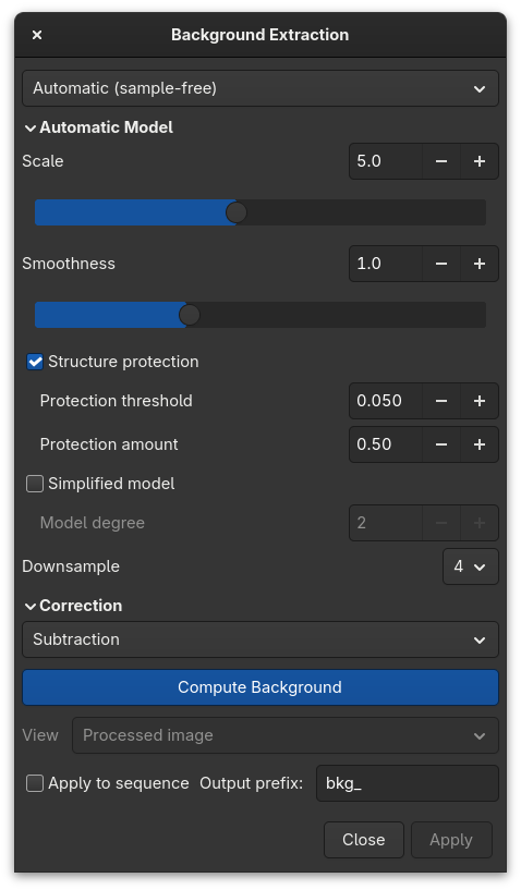
Background extraction dialog with the automatic (sample-free) method selected, showing the Automatic Model panel.

Advertencia

The automatic method fits the background over the whole image, borders included. Stacked images very often have black or uneven edges (caused by dithering, field rotation or incomplete overlap between frames). These borders must be cropped away before running the automatic method, otherwise they are treated as extremely dark background and corrupt the model. Unlike the sample-based method, the edges cannot be excluded here by making a selection, so a clean crop of the stacked result is imperative.

The following parameters are available in the Automatic Model panel:

• Scale: relative scale of the multiscale model, in the [1, 10] range (default 5). A higher value keeps only large-scale gradients and gives a smoother model, while a lower value lets the model follow more complex or more local gradients.

• Smoothness: extra smoothing applied to the final model (default 1). A higher value gives a softer, more gradual background; a value of 0 leaves the fitted model untouched.

• Structure protection: when enabled (the default), extended bright structures such as nebulae are masked so that they are not absorbed into the background model. Two sub-parameters control it:

  • Protection threshold: brightness above the model at which a pixel starts to be treated as a structure (default 0.05). A lower value protects more of the image.

  • Protection amount: how far the protection mask grows around the detected structures (default 0.5).

• Simplified model: replaces the multiscale model with a stiff low-degree polynomial. Use it when a nebula fills most of the frame and the default model would hollow it out. Its degree is set with:

  • Model degree: polynomial degree of the simplified model, in the [1, 6] range (default 2). A lower value is stiffer (degree 1 is a plane).

• Downsample: internal working scale factor (1, 2, 4 or 8, default 4). A higher value makes the computation faster but coarser; it does not change the scale of the background itself.

Truco

Start with the default settings. If real signal (a large nebula) is being eaten by the model, either lower the Protection threshold or switch to the Simplified model with a low Model degree.

Theory

The automatic model is estimated independently on each channel and, for speed, on an internally downsampled copy of the image (the Downsample factor). It then alternates a fit step and a robust rejection step:

1. An initial background model \(B\) is fitted on every pixel.

2. The residual \(r = I - B\) between the image \(I\) and the current model is computed, and its robust location and scale are estimated from the pixels currently kept, using the median and the median absolute deviation (\(\sigma = 1.4826 \times \mathrm{MAD}\)).

3. Pixels are rejected by an asymmetric sigma clipping: a pixel is kept only if its residual lies within \([\,\mathrm{med} - k_\mathrm{lo}\,\sigma,\ \mathrm{med} + k_\mathrm{hi}\,\sigma\,]\), with a tighter upper bound than the lower one. Bright outliers (stars, nebula cores) are therefore discarded more aggressively than faint ones.

4. When Structure protection is enabled, a spatially-coherent mask of extended bright structures is additionally removed from the fitting set, so large nebulae are not mistaken for background.

5. The model is re-fitted on the surviving pixels and the process repeats until the kept set stabilises.

Two models are available. The default multiscale model rebuilds a smooth surface across the rejected regions by harmonic-style inpainting (repeated low-pass filtering that restores the kept pixels at each pass); the Scale parameter sets the width of that low-pass, i.e. the spatial scale below which variations are considered signal rather than background. The simplified model instead fits a single 2D polynomial of the chosen Model degree by least squares. In both cases a final, optional Gaussian smoothing is controlled by Smoothness.

The low-pass filtering relies on a fast separable Gaussian approximated by variance-matched box blurs, so its cost is independent of the smoothing radius.

General settings

These controls sit below the method panels and apply whichever method is selected.

• Correction:

  • Subtraction: it is mainly used to correct additive effects, such as gradients caused by light pollution or by the Moon.

  • Division: it is mainly used to correct multiplicative phenomena, such as vignetting or differential atmospheric absorption for example. However, this kind of operation should be done by master-flat correction.

• Compute Background: This will compute the synthetic background and will apply the selected correction. The model is always computed from the original image kept in memory allowing the user to work iteratively. The result is only previewed at this stage; it is committed when you close the dialog with the Apply button.

• View: once a background has been computed, this drop-down chooses what is shown in the main view without recomputing anything:

  • Processed image: the corrected result (the default).

  • Background model: the background that was removed, reconstructed from the original and the processed image.

  • Original image: the untouched image kept in memory.

  This replaces the former Show original image button and works identically for both methods.

The background gradient of pre-processed image can be complex because the gradient may have rotated with the acquisition session. It can be difficult to completely remove it, because it’s difficult to represent it with a polynomial function. If this is the case, you may consider removing the gradient in the subexposures: in a single image, the background gradient is much simpler and generally follows a simple linear (degree 1) function.

Truco

Sometimes unsightly color banding appears after background extraction. When this happens, there are two things to check. Firstly, if the image is in 16-bit, we strongly advise you to always use the 32-bit format. If, despite everything, you still observe such artifacts, the add dither option, explained above, is the solution to your problem.

When such banding occurs after gradient extraction. It can be solved with the add dither option (Courtesy of Nathan B.).

Truco

Good results with the RBF algorithm generally require fewer samples than with the polynomial algorithm.

Ver también

For more explanations, see the corresponding tutorial here.

Siril command line

subsky { -rbf | degree } [-dither] [-samples=20] [-tolerance=1.0] [-smooth=0.5] [-existing] [-random] [-gradient] [-border=<pixels|percent%>]

Computes a synthetic background gradient using either the polynomial function model of degree degrees or the RBF model (if -rbf is provided instead) and subtracts it from the image.

The number of samples per horizontal line and the tolerance to exclude brighter areas can be adjusted with the optional arguments. Tolerance is in MAD units: median + tolerance * mad.

Dithering, required for low dynamic gradients, can be enabled with -dither.

For RBF, the additional smoothing parameter is also available. To use pre-existing background samples (e.g. if you have set background samples using a Python script) the -existing argument must be used.

-random: place sample points randomly in darker areas of each image quadrant plus fixed border/corner points, instead of using a regular grid. In this mode the -samples value is the total number of interior random points.

-gradient: after placing each sample (grid or random), move it to the nearest local brightness minimum using gradient descent, shifting it away from stars and other bright objects. Can be combined with either placement mode.

-border=: exclude a border strip from sample placement. For a pixel value (e.g. -border=50), the same number of pixels is excluded from all four sides. For a percentage value (e.g. -border=10%), the left and right strips are that percentage of the image width, and the top and bottom strips are that percentage of the image height, so the excluded area is proportional to the image dimensions rather than a fixed pixel count

Truco

The automatic (sample-free) method is available on the command line with the -auto argument. In this mode the sample-related options are ignored and the automatic-model parameters (-scale=, -smoothness=, -noprotect, -protect_threshold=, -protect_amount=, -simplified, -degree=, -downsample=) apply instead, together with -mode=subtract|divide for the correction type. See the subsky reference above for the full list.

Truco

The -existing command argument forces use of existing background samples. This option is primarily for use in conjunction with the Python module where SirilInterface.set_bgsamples() can be used to set custom background samples based on user-defined algorithms. If it is not provided, subsky will automatically regenerate background samples. Note that the -existing option is not available with the seqsubsky command, because sequence frames are not necessarly registered at the time background subtraction is carried out, so the samples for one frame do not necessarily apply to another.

Siril command line

seqsubsky sequencename { -rbf | degree } [-nodither] [-samples=20] [-tolerance=1.0] [-smooth=0.5] [-prefix=] [-random] [-gradient] [-border=<pixels|percent%>]

Same command as SUBSKY but for the sequence sequencename.

Dithering, required for low dynamic gradients, can be disabled with -nodither. Note that the -existing option is not available for sequence background removal, as the frames of a sequence are not necessarily always aligned.

The output sequence name starts with the prefix "bkg_" unless otherwise specified with -prefix= option. Only selected images in the sequence are processed.

-random and -gradient options are available as in SUBSKY.

-border= is available as in SUBSKY

Links: subsky

[Wright2003]

Wright, Grady Barrett. Radial basis function interpolation: numerical and analytical developments. University of Colorado at Boulder, 2003.